Download
1 / 72
730 likes | 760 Views
Deep Inelastic Scattering (DIS) CTEQ School ’08- Debrecen A.M.Cooper-Sarkar Oxford What have we learnt from DIS in the last 30 years? QPM, QCD Parton Distribution Functions, alpha_s Low-x physics Electroweak. PDFs were first investigated in deep inelastic lepton-hadron scatterning -DIS.

E N D
Deep Inelastic Scattering (DIS) CTEQ School ’08- Debrecen A.M.Cooper-Sarkar Oxford What have we learnt from DIS in the last 30 years? QPM, QCD Parton Distribution Functions, alpha_s Low-x physics Electroweak
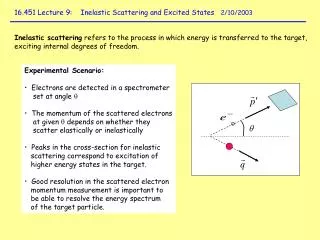
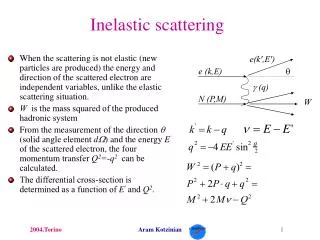
PDFs were first investigated in deep inelastic lepton-hadron scatterning -DIS Leptonic tensor - calculable 2 Lμν Wμν dσ~ Hadronic tensor- constrained by Lorentz invariance Et q = k – k’, Q2 = -q2 Px = p + q , W2 = (p + q)2 s= (p + k)2 x = Q2 / (2p.q) y = (p.q)/(p.k) W2 = Q2 (1/x – 1) Q2 = s x y Ee Ep s = 4 Ee Ep Q2 = 4 Ee E’ sin2θe/2 y = (1 – E’/Ee cos2θe/2) x = Q2/sy The kinematic variables are measurable
Completely generally the double differential cross-section for e-N scattering d2(e±N) = [ Y+ F2(x,Q2) - y2 FL(x,Q2) ± Y_xF3(x,Q2)], Y± = 1 ± (1-y)2 dxdy Leptonic part hadronic part F2, FL and xF3 are structure functionswhich express the dependence of the cross-section on the structure of the nucleon– The Quark-Parton model interprets these structure functions as related to the momentum distributions of quarks or partons within the nucleon AND the measurable kinematic variablex = Q2/(2p.q)is interpreted as the FRACTIONAL momentum of the incoming nucleon taken by the struck quark (xP+q)2=x2p2+q2+2xp.q ~ 0 for massless quarks and p2~0so x = Q2/(2p.q) The FRACTIONAL momentum of the incoming nucleon taken by the struck quark is the MEASURABLE quantity x e.g. for charged lepton beams F2(x,Q2) = Σi ei2(xq(x) + xq(x)) – Bjorken scaling FL(x,Q2) = 0 - spin ½ quarks xF3(x,Q2) = 0 - only γexchange However for neutrino beams xF3(x,Q2)= Σi (xq(x) - xq(x)) ~ valence quark distributions of various flavours
Consider electron muon scattering ds = 2pa2s [ 1 + (1-y)2] , for elastic eμ dy Q4 isotropic non-isotropic ds = 2pa2ei2 s [ 1 + (1-y)2] , so for elastic electron quark scattering, quark charge ei e dy Q4 d2s= 2pa2 s [ 1 + (1-y)2] Σiei2(xq(x) + xq(x)) so for eN, where eq has c. of m. energy2 equal toxs, and q(x) gives probability that such a quark is in the Nucleon dxdy Q4 Now compare the general equation to the QPM prediction to obtain the results F2(x,Q2) = Σiei2(xq(x) + xq(x)) – Bjorken scaling – this depends only on x FL(x,Q2) = 0 - spin ½ quarks xF3(x,Q2) = 0 - only γexchange
Consider n,n scattering: neutrinos are handed ds(n)= GF2 x s ds(n) = GF2 x s (1-y)2 Compare to the general form of the cross-section for n/n scattering via W+/- FL(x,Q2) = 0 xF3(x,Q2) = 2Σix(qi(x) - qi(x)) Valence F2(x,Q2) = 2Σix(qi(x) + qi(x)) Valence and Sea And there will be a relationship between F2eN and F2nN Also NOTE n,n scattering is FLAVOUR sensitive dy p dy p For nq (left-left) For n q (left-right) d2s(n) = GF2 s Σi [xqi(x) +(1-y)2xqi(x)] dxdy p For nN d2s(n) = GF2 s Σi [xqi(x) +(1-y)2xqi(x)] dxdy p For nN Clearly there are antiquarks in the nucleon 3 Valence quarks plus a flavourless qq Sea m- W+ can only hit quarks of charge -e/3 or antiquarks -2e/3 n W+ u d s(np)~ (d + s) + (1- y)2 (u + c) s(np) ~ (u + c) (1- y)2 + (d + s) q = qvalence +qsea q = qsea qsea= qsea
So in n,n scattering the sums over q, qbar ONLY contain the appropriate flavours BUT- high statistics n,n data are taken on isoscalar targets e.g. Fe Y (p + n)/2=N d in proton = u in neutron u in proton = d in neutron GLS sum rule Total momentum of quarks A TRIUMPH (and 20 years of understanding the c c contribution)
BUT – Bjorken scaling is broken F2 does not depend only on x it also depends on Q2 – ln(Q2) Particularly strongly at small x
QCD improves the Quark Parton Model What if or x x Pqq Pgq y y Before the quark is struck? Pqg Pgg y > x, z = x/y So F2(x,Q2) = Σi ei2(xq(x,Q2) + xq(x,Q2)) in LO QCD The theory predicts the rate at which the parton distributions (both quarks and gluons) evolve with Q2- (the energy scale of the probe) -BUT it does not predict their shape The DGLAP parton evolution equations
What if higher orders are needed? Note q(x,Q2) ~ αs lnQ2, but αs(Q2)~1/lnQ2, so αs lnQ2 is O(1), so we must sum all terms αsn lnQ2n Leading Log Approximation x decreases from ss(Q2) target to probe xi-1> xi > xi+1…. Pqq(z) = P0qq(z) + αs P1qq(z) +αs2 P2qq(z) LO NLO NNLO pt2 of quark relative to proton increases from target to probe pt2i-1 < pt2i < pt2i+1 Dominant diagrams have STRONG pt ordering F2 is no longer so simply expressed in terms of partons - convolution with coefficient functions is needed – but these are calculable in QCD FL is no longer zero.. And it depends on the gluon
How do we determine Parton Distribution Functions ? Parametrise the parton distribution functions (PDFs) at Q20 (~1-7 GeV2)- Use NLO QCD DGLAP equations to evolve these PDFs to Q2 >Q20 Construct the measurable structure functions and cross-sections by convoluting PDFs with coefficient functions: make predictions for ~2000 data points across the x,Q2 plane- Perform χ2 fit to the data Who? Alekhin, CTEQ, MRST, H1, ZEUS http://durpdg.dur.ac.uk/hepdata/ http://projects.hepforge.org/lhapdf/ Formalism NLO DGLAP MSbar factorisation Q02 functional form @ Q02 sea quark (a)symmetry etc. fi (x,Q2) fi (x,Q2) αS(MZ ) Data DIS (SLAC, BCDMS, NMC, E665, CCFR, H1, ZEUS, CCFR, NuTeV ) Drell-Yan (E605, E772, E866, …) High ET jets (CDF, D0) W rapidity asymmetry (CDF) etc. LHAPDFv5
The DATA – the main contribution is DIS data Terrific expansion in measured range across the x, Q2 plane throughout the 90’s HERA data Pre HERA fixed target p,D NMC, BDCMS, E665 and ,bar Fe CCFR We have to impose appropriate kinematic cuts on the data so as to remain in the region when the NLO DGLAP formalism is valid • Q2 cut : Q2 > few GeV2 so that perturbative QCD is applicable- αs(Q2) small • W2 cut: to avoid higher twist terms- usual formalism is leading twist • x cut: to avoid regions where ln(1/x) resummation (BFKL) and non-linear effects may be necessary….
Need to extend the formalism? Optical theorem 2 The handbag diagram- QPM Im QCD at LL(Q2) Ordered gluon ladders (αsn lnQ2 n) NLL(Q2) one rung disordered αsn lnQ2 n-1 ? BUT what about completely disordered Ladders? at small x there may be a need for BFKLln(1/x) resummation? And what about Higher twist diagrams ? Are they always subdominant? Important at high x, low Q2
The strong rise in the gluon density at small-x leads to speculation that there may be a need for non-linear equations?- gluons recombining gg→g Non-linear fan diagrams form part of possible higher twist contributions at low x- no sign of these in data
The CUTS In practice it has been amazing how low in Q2 the standard formalism still works- down to Q2 ~ 1 GeV2 : cut Q2 > 2 GeV2 is typical It has also been surprising how low in x – down to x~ 10-5 : no x cut is typical Nevertheless there are doubts as to the applicability of the formalism at such low-x.. (See later) there could beln(1/x) corrections and/or non-linear high density corrections for x < 5 10 -3
Higher twist terms can be important at low-Q2 and high-x→ this is the fixed target region (particularly SLAC- and now JLAB data). Kinematic target mass corrections and dynamic contributions ~ 1/Q2 X→ 2x/(1 + √(1+4m2x2/Q2)) Fit with F2=F2LT (1 +D2(x)/Q2) Fits establish that higher twist terms are not needed if W2 > 15 GeV2 – typical W2 cut
The form of the parametrisation Parametrise the parton distribution functions (PDFs) at Q20 (~1-7 GeV2) Parameters Ag, Au, Ad are fixed through momentum and number sum rules– explain other parameters may be fixed by model choices- Model choices Form of parametrization at Q20, value ofQ20,, flavour structure of sea, cuts applied, heavy flavour scheme → typically ~15-22 parameters Use QCD to evolve these PDFs to Q2 >Q20 Construct the measurable structure functions by convoluting PDFs with coefficient functions: make predictions for ~2000 data points across the x,Q2 plane Perform χ2 fit to the data xuv(x) =Auxau (1-x)bu (1+ εu√x + γu x) xdv(x) =Adxad (1-x)bd (1+ εd√x + γdx) xS(x) =Asx-λs (1-x)bs (1+ εs√x + γsx) xg(x) =Agx-λg(1-x)bg (1+ εg√x + γgx) These parameters control the low-x shape These parameters control the middling-x shape These parameters control the high-x shape Alternative form for CTEQ xf(x) = A0xA1(1-x)A2 eA3x (1+eA4x)A5 The fact that so few parameters allows us to fit so many data points established QCD as the THEORY OF THE STRONG INTERACTION and provided the first measurements of s (as one of the fit parameters)
The form of the parametrisationat Q20 Ultimately we may get this from lattice QCD, or other models- the statistical model is quite successful (Soffer et al). But we can make some guesses at the basic form: xa (1-x)b ….. at one time (20 years ago?) we thought we understood it! --------the high x power from counting rules ----(1-x)2ns-1 - ns spectators valence (1-x)3, sea (1-x)7, gluon (1-x)5 --------the low-x power from Regge – low-x corresponds to high centre of massenergy for the virtual boson proton collision (x = Q2 / (2p.q)) -----Regge theory gives high energy cross-sections as s (α-1) -----------which gives x dependence x (1-α), where α is the intercept of the Regge trajectory- different for singlet (no overall flavour) F2 ~x0 and non-singlet (flavour- valence-like) xF3~x0.5 The shapes of F2 and xF3 even looked like this – pre HERA
But at what Q2 would these be true? – Valence distributions evolve slowly but sea and gluon distributions evolve fast– we are just parametrising our ignorance -----and we need the arbitrary polynomial In any case the further you evolve in Q2 the less the parton distributions look like the low Q2 inputs and the more they are determined by QCD evolution –Valence distributions evolve slowly Sea/Gluon distributions evolve fast Some people don’t use a starting parametrization at all- but let neural nets learn the shape of the data- NNPDF
Where is the information coming from? • Originally- pre HERA • Fixed target e/μ p/D data from NMC, BCDMS, E665, SLAC • F2(e/p)~ 4/9 x(u +ubar) +1/9x(d+dbar) + 4/9 x(c +cbar) +1/9x(s+sbar) • F2(e/D)~5/18 x(u+ubar+d+dbar) + 4/9 x(c +cbar) +1/9x(s+sbar) • Also use ν, νbar fixed target data from CCFR( now also NuTeV/Chorus) (Beware Fe target needs nuclear corrections) • F2(ν,νbar N) = x(u +ubar + d + dbar + s +sbar + c + cbar) • xF3(ν,νbar N) = x(uv + dv ) (provided s = sbar) • Valence information for 0< x < 1 • Can get ~4 distributions from this: e.g. u, d, ubar, dbar – but need assumptions • like q=qbar for all flavours, sbar = 1/4 (ubar+dbar), dbar = ubar (wrong!) and need heavy quark treatment. • Note gluon enters only indirectly via DGLAP equations for evolution Assuming u in proton = d in neutron – strong-isospin
Flavour structure Historically an SU(3) symmetric sea was assumed u=uv+usea, d=dv+dsea usea= ubar = dsea = dbar = s = sbar =K and c=cbar=0 Measurements of F2μn = uv + 4dv +4/3K F2μp 4uv+ dv +4/3K Establish no valence quarks at small-x F2μn/F2μp→1 But F2μn/F2μp →1/4 as x → 1 Not to 2/3 as it would for dv/uv=1/2, hence it look s as if dv/uv →0 as x →1 i.e the dv momentum distribution is softer than that of uv- Why? Non-perturbative physics --diquark structures? How accurate is this? Could dv/uv →1/4 (Farrar and Jackson)?
Flavour structure in the sea dbar ≠ubar in the sea Consider the Gottfried sum-rule (at LO) ∫ dx (F2p-F2n) = 1/3 ∫dx (uv-dv) +2/3∫dx(ubar-dbar) If ubar=dbar then the sum should be 0.33 the measured value from NMC = 0.235 ± 0.026 Clearly dbar > ubar…why? low Q2 non-perturbative effects, Pauli blocking, p →nπ+,pπ0,Δ++π- m- sbar≠(ubar+dbar)/2, in fact sbar ~ (ubar+dbar)/4 Why? The mass of the strange quark is larger than that of the light quarks Evidence – neutrino opposite sign dimuon production rates And even s≠sbar? Because of p→ΛK+ n W+ c→s μ+ s
So what did HERA bring? Low-x – within conventional NLO DGLAP Before the HERA measurements most of the predictions for low-x behaviour of the structure functions and the gluon PDF were wrong HERA ep neutral current (γ-exchange) data give much more information on the sea and gluon at small x….. xSea directly from F2, F2 ~ xq xGluon from scaling violations dF2 /dlnQ2 – the relationship to the gluon is much more direct at small-x, dF2/dlnQ2 ~ Pqgxg
Low-x t = ln Q2/2 Gluon splitting functions become singular αs ~ 1/ln Q2/2 At small x, small z=x/y A flat gluon at low Q2 becomes very steep AFTER Q2 evolution AND F2 becomes gluon dominated F2(x,Q2) ~ x -λs, λs=λg -ε xg(x,Q2) ~ x -λg
High Q2 HERA data-still to be fully exploited HERA data have also provided information at high Q2→ Z0 and W+/- become as important as γexchange → NC and CC cross-sections comparable For NC processes F2= i Ai(Q2) [xqi(x,Q2) + xqi(x,Q2)] xF3= iBi(Q2) [xqi(x,Q2) - xqi(x,Q2)] Ai(Q2) = ei2 – 2 eivi vePZ + (ve2+ae2)(vi2+ai2) PZ2 Bi(Q2) = – 2 eiai ae PZ + 4ai ae vi ve PZ2 PZ2 = Q2/(Q2 + M2Z) 1/sin2θW a new valence structure function xF3 due to Z exchange is measurable from low to high x- on a pure proton target → no heavy target corrections- no assumptions about strong isospin
CC processes give flavour information d2(e+p) = GF2 M4W [x (u+c) + (1-y)2x (d+s)] d2(e-p) = GF2 M4W [x (u+c) + (1-y)2x (d+s)] dxdy 2x(Q2+M2W)2 dxdy 2x(Q2+M2W)2 uv at high x dv at high x MW information Measurement of high-x dvon a pure proton target d is not well known because u couples more strongly to the photon. Historically information has come from deuterium targets –but even Deuterium needs binding corrections. Open questions: does u in proton = d in neutron?, does dv/uv 0, as x 1?
To reveal the difference in both large and small x regions To view small and large x in one plot The u quark LO fits to early fixed-target DIS data
Gluon HERA steep rise of F2 at low x
Gluon More recent fits with HERA data- steep rise even for low Q2 ~ 1 GeV2 Tev jet data Does gluon go negative at small x and low Q?seeMRST/W PDFs
Recent development: Combining ZEUS and H1 data sets • Not just statistical improvement. Each experiment can be used to calibrate the othersince they have rather different sources of experimental systematics • Before combination the systematic errors are ~3 times the statistical for Q2< 100 • After combination systematic errors are < statistical
PDF comparison 2008 HERAPDF0.1 gives very small experimental errors and modest model errors
End lecture 1 • Next PDFs for the LHC • Beware of low-x physics
The Standard Model is not as well known as you might think fa pA x1 • where X=W, Z, D-Y, H, high-ET jets, prompt-γ • and is known • to some fixed order in pQCD and EW • in some leading logarithm approximation (LL, NLL, …) to all orders via resummation ^ pB x2 fb X Knowledge from HERA →the LHC- transport PDFs to hadron-hadron cross-sections using QCD factorization theorem for short-distance inclusive processes The central rapidity range for W/Z production AT LHC is at low-x (5 ×10⁻⁴ to 5 ×10⁻²)
Look at predictions for W/Z rapidity distributions Pre- and Post-HERA Why such an improvement? Pre HERA Post HERA It’s due to the improvement in the low-x gluon At the LHC the q-qbar which make the boson are mostly sea-sea partons at low-x And at Q2~MZ2 the sea is driven by the gluon
This is post HERA but just one experiment This is post HERA using the new (2008) HERA combined PDF fit
BEWARE of different sort of ‘new physics’ LHC is a low-x machine (at least for the early years of running) Low-x information comes from evolving the HERA data Is NLO (or even NNLO) DGLAP good enough? The QCD formalism may need extending at small-x BFKL ln(1/x) resummation High density non-linear effects etc. (Devenish and Cooper-Sarkar, ‘Deep Inelastic Scattering’, OUP 2004, Section 6.6.6 and Chapter 9 for details!)
Before the HERA measurements most of the predictions for low-x behaviour of the structure functions and the gluon PDF were wrong Now it seems that the conventional NLO DGLAP formalism works TOO WELL _ there should beln(1/x) corrections and/or non-linear high density corrections for x < 5 10 -3
Low-x t = ln Q2/2 Gluon splitting functions become singular αs ~ 1/ln Q2/2 At small x, small z=x/y A flat gluon at low Q2 becomes very steep AFTER Q2 evolution AND F2 becomes gluon dominated F2(x,Q2) ~ x -λs, λs=λg -ε xg(x,Q2) ~ x -λg
So it was a surprise to see F2 steep at small x - for low Q2, Q2 ~ 1 GeV2 Should perturbative QCD work? αs is becoming large - αs at Q2 ~ 1 GeV2 is ~ 0.4
Need to extend formalism at small x? The splitting functions Pn(x), n= 0,1,2……for LO, NLO, NNLO etc Have contributions Pn(x) = 1/x [ an ln n (1/x) + bn ln n-1 (1/x) …. These splitting functions are used in evolution dq/dlnQ2 ~ s dy/y P(z) q(y,Q2) And thus give rise to contributions to the PDF sp (Q2) (ln Q2)q (ln 1/x) r DGLAP sums- LL(Q2) and NLL(Q2) etc STRONGLY ordered in pt. But if ln(1/x) is large we should consider Leading Log 1/x (LL(1/x)) and Next to Leading Log (NLL(1/x)) - BFKL summations LL(1/x) is STRONGLY ordered in ln(1/x) and can be disordered in pt BFKL summation at LL(1/x) xg(x) ~ x -λ λ = αs CA ln2 ~ 0.5 steep gluon even at moderate Q2 Disordered gluon ladders But NLL(1/x) softens this somewhat
The steep behaviour of the gluon is deduced from the DGLAP QCD formalism – BUT the steep behaviour of the low-x Sea can be measured from F2 ~ x -λs, λs = d ln F2 d ln 1/x Small x is high W2, x=Q2/2p.q = Q2/W2. At small x б(γ*p) = 4π2α F2/Q2 F2 ~ x –λs → б (γ*p) ~ (W2)λs Buts(g*p) ~ (W2) α-1 – is the Regge prediction for high energy cross-sections where α is the intercept of the Regge trajectory α=1.08 for the SOFT POMERON Such energy dependence is well established from the SLOW RISE of all hadron-hadron cross-sections - including s(gp) ~ (W2) 0.08 for real photon- proton scattering Obviously the virtual-photon proton cross-section only obeys the Regge prediction for Q2 < 1. Does the steeper rise of б (γ*p)require a HARD POMERON? --The BFKL Pomeron with alpha=1.5 ? What about the Froissart bound?
Furthermore if the gluon density becomes large there maybe non-linear effects Gluon recombination g g g ~ αs22/Q2 may compete with gluon evolution g g g ~ αs where is the gluon density ~ xg(x,Q2) –no.of gluons per ln(1/x) Colour Glass Condensate, JIMWLK, BK nucleon size R2 Non-linear evolution equations – GLR d2xg(x,Q2) = 3αs xg(x,Q2) – αs2 81 [xg(x,Q2)]2 Higher twist dlnQ2dln1/x π 16Q2R2 αs αs22/Q2 The non-linear term slows down the evolution of xg(x,Q2) and thus tames the rise at small x The gluon density may even saturate (-respecting the Froissart bound) Extending the conventional DGLAP equations across the x, Q2 plane Plenty of debate about the positions of these lines!
Do the data NEED unconventional explanations ? In practice the NLO DGLAP formalism works well down to Q2 ~ 1 GeV2 BUT below Q2 ~ 5 GeV2 the gluon is no longer steep at small x – in fact its becoming negative! xS(x) ~ x –λs, xg(x) ~ x –λg λg < λs at low Q2, low x So far, we only used F2 ~ xq dF2/dlnQ2 ~ Pqgxg Unusual behaviour of dF2/dlnQ2 may come from unusual gluon or from unusual Pqg- alternative evolution?. Non-linear effects? We need other gluon sensitive measurements at low x, like FL or F2charm…. `Valence-like’ gluon shape
But charm is not so simple to calculate Heavy quark treatments differ Massive quarks introduce another scale into the process, the approximation mq2~0 cannot be used Zero Mass Variable Flavour Number Schemes (ZMVFNs) traditional c=0 until Q2 ~4mc2, then charm quark is generated by g→ c cbar splitting and treated as massless-- disadvantage incorrect to ignore mc near threshold Fixed Flavour Number Schemes (FFNs) If W2 > 4mc2 then c cbar can be produced by boson-gluon fusion and this can be properly calculated - disadvantage ln(Q2/mc2) terms in the cross-section can become large- charm is never considered part of the proton however high the scale is. General Mass variable Flavour Schemes (GMVFNs) Combine correct threshold treatment with resummation of ln(Q2/mc2) terms into the definition of a charm quark density at large Q2 Arguments as to correct implementation but should look like FFN at low scale and like ZMVFN at high scale. Additional complications for W exchange s→c threshold.
We are learning more about heavy quark treatments than about the gluon, so far
And now we have actually measured FL! FL looks pretty conventional- can be described with usual NLO DGLAP formalism But see later (Thorne and White)
No smoking gun for something new at low-x…so let’s look more exclusively Let’s look at jet production:First let’s just see what jets can do for us in a regular NLO DGLAP fit There is a decrease in gluon PDF uncertainty from using jet data in PDF fits Direct* Measurement of the Gluon Distribution ZEUS-jets PDF fit
Before jets After jets And correspondingly the contribution of the uncertainty onαs(MZ) to the uncertainty on the PDFs is much reduced Nice measurement of αs(MZ) = 0.1183 ± 0.0028 (exp) ± 0.0008 (model) From simultaneous fit of αs(MZ) & PDF parameters And use of jet data can help to tie down both alphas itself and alphas related uncertainties on the gluon PDF