Download
1 / 22
250 likes | 367 Views
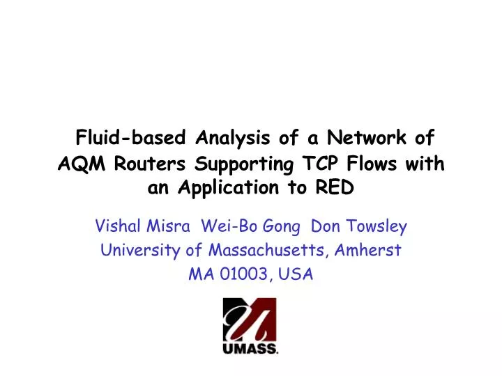
Fluid-based Analysis of a Network of AQM Routers Supporting TCP Flows with an Application to RED. Vishal Misra Wei-Bo Gong Don Towsley University of Massachusetts, Amherst MA 01003, USA. Overview. motivation key idea modeling details experimental validation with ns

E N D
Fluid-based Analysis of a Network of AQM Routers Supporting TCP Flows with an Application to RED Vishal Misra Wei-Bo Gong Don Towsley University of Massachusetts, Amherst MA 01003, USA
Overview • motivation • key idea • modeling details • experimental validation with ns • analysis sheds insights into RED • Conclusions
Motivation • current simulation technology, e.g. ns • appropriate for small networks 10s - 100s of network nodes 100s - 1000s IP flows • inflexible packet-level granularity • current analysis technology • UDP flows over small networks • TCP flows over single link ... ... ...
Challenge Need to explore systems with a parameter space of: • 100s - 1000s network elements • 10,000s - 100,000s of flows (TCP, UDP, NG) Belief Fluid based simulation techniques which abstract out and exploit topologies/protocols are key for scalability Contribution of Paper First differential equation based fluid model to enable transient analysis of TCP/AQM networks developed
Key Idea • model traffic as fluid • describe behavior of flows and queues using Stochastic Differential Equations • obtain Ordinary Differential Equations by taking expectations of the SDEs • solve the resultant coupled ODEs numerically Differential equation abstraction: computationally highly efficient
Packet Drop/Mark Round Trip Delay (t) Loss Model AQM Router B(t) p(t) Sender Receiver Loss Rate as seen by Sender: l(t) = B(t-t)*p(t-t)
A Single Congested Router • N TCP flows • window sizes Wi(t) • round trip time Ri(t) = Ai+q(t)/C • throughputs Bi(t) = Wi(t)/Ri(t) • One bottlenecked AQM router • capacity {C (packets/sec)} • queue length q(t) • discard prob. p(t) TCP flow i AQM router C, p
- q(t) - x(t) discontinuity removed in gentle_ variant t -> 2tmax Adding RED to the model RED: Marking/dropping based on average queue length x(t) Marking probability profile has a discontinuity at tmax 1 Marking probability p pmax tmin tmax Average queue length x x(t): smoothed, time averaged q(t)
^ ^ dWi dt Wi 2 1 = - Mult. decrease Loss arrival rate Additive increase ^ Queue length: ^ Ri(q(t)) ^ dq dt -1[q(t) > 0]C + S = ^ ^ Wi(t-t) ^ ^ ^ p(t-t) Outgoing traffic Incoming traffic ^ Ri(q(t)) Ri (q(t-t)) ^ Wi(t) System of Differential Equations All quantities are average values. Timeouts and slow start ignored Window Size:
^ Average queue length: Where a = averaging parameter of RED(wth) d = sampling interval ~ 1/C dx dt x(t) ^ - = ln (1-a) ln (1-a) ^ ^ dp dt dp dx dx dt = Loss probability: d d Where dp is obtained from the marking profile dx q(t) ^ System of Differential Equations (cont.)
N+2 coupled equations ^ dq/dt =f2(Wi) ^ dp/dt = f3(q) ^ ^ N flows Wi(t) = Window size of flow i Ri(t) = RTT of flow i p(t) = Drop probability q(t) = queue length dWi/dt = f1(p,Ri, Wi) i =1..N ^ ^ ^ ^ Equations solved numerically using MATLAB
Extension to Network Networked case: V congested AQM routers queuing delay = aggregate delay q(t) = SV qV(t) loss probability = cumulative loss probability p(t) = 1-PV(1-pV(t)) Other extensions to the model Timeouts: Leveraged work done in [PFTK Sigcomm98] to model timeouts Aggregation of flows: Represent flows sharing the same route by a single equation
Flow set 4 Flow set 1 RED router 1 Flow set 2 Flow set 3 Flow set 5 Experimental scenario Topology • DE system programmed with RED AQM policy • equivalent system programmed in ns • transient queuing performance obtained • one way, ftp flows used as traffic model RED router 2 5 sets of flows 2 RED routers Set 2 flows through both routers
Performance of SDE method • queue capacity 5 Mb/s • load variation at t=75 and t=150 seconds • 200 flows simulated • DE solver captures transient performance • time taken for DE solver ~ 5 seconds on P450 DE method ns simulation Queue length Time
Observations on RED • RED behavior changes with change in network conditions (load level, packet size, link bandwidth). “Tuning” of RED is difficult, queue length frequently oscillates deterministically. • discontinuity of drop function contributes to, but is not the only reason for oscillations. • RED uses a variable d (sampling interval). This variable sampling could cause oscillations. • averaging mechanism of RED is counter productive from stability viewpoint: introduces a further delay to the existing round trip delay.
Future Direction • model short lived and non-responsive flows • demonstrate applicability to large networks • analyze theoretical model to rectify REDshortcomings • apply techniques to other “TCP-like” protocols, e.g. equation based TCP-friendlyprotocols
Conclusions • differential equation based model for TCP/AQM networks developed • computation cost of DE method a fraction of the discrete event simulation cost • formal representation and analysis yields better understanding of RED/AQM
Loss Indications arrival rate l Traditional, Source centric loss model New, Network centric loss model Sender New loss model proposed in “Stochastic Differential Equation Modeling and Analysis of TCP Window size behavior”, Misra et. al. Performance 99. Sender Loss Probability pi Loss model enabled casting of TCP behavior as a Stochastic Differential Equation dw = dt/R-w/2dNtd+(1-w)dNto Background
Networkis a (blackbox) source of R and l l R l R Solution: Express R and l as functions of B Network Deficiency of earlier Model Throughput (B(t)) is a function of loss rate (l) and round trip time (R) B(t) = f(l,R)
- q(t) - x(t) - q(t) - x(t) t -> t ->
System of Differential Equations All quantities are expectedvalues. We ignore timeouts and slowstart in this formulation. Window size: Queue length: dq =-1[q(t) > 0] Cdt + SWi(t)/Ri(q(t))dt Average Queue size: dx = ln (1-a)/d x(t) - ln (1-a)/d q(t) Where a= averaging parameter of RED (wth) d= sampling interval ~ 1/C