Download
1 / 128
1.28k likes | 1.45k Views
Evolutionary Computation ( 진 화 연 산 ). 장 병 탁 서울대 컴퓨터공학부 E-mail: btzhang@cse.snu.ac.kr http://scai.snu.ac.kr./~btzhang/ Byoung-Tak Zhang School of Computer Science and Engineering Seoul National University This material is also available online at http://scai.snu.ac.kr/. Outline.

E N D
Evolutionary Computation(진 화 연 산) 장 병 탁 서울대 컴퓨터공학부 E-mail: btzhang@cse.snu.ac.kr http://scai.snu.ac.kr./~btzhang/ Byoung-Tak Zhang School of Computer Science and Engineering Seoul National University This material is also available online at http://scai.snu.ac.kr/
Outline • Basic Concepts • Theoretical Backgrounds • Applications • Current Issues • References and URLs
Charles Darwin (1859) “Owing to this struggle for life, any variation, however slight and from whatever cause proceeding, if it be in any degree profitable to an individual of any species, in its infinitely complex relations to other organic beings and to external nature, will tend to the preservation of that individual, and will generally be inherited by its offspring.”
Evolutionary Algorithms • A Computational Model Inspired by Natural Evolution and Genetics • Proved Useful for Search, Machine Learning and Optimization • Population-Based Search (vs. Point-Based Search) • Probabilistic Search (vs. Deterministic Search) • Collective Learning (vs. Individual Learning) • Balance of Exploration (Global Search) and Exploitation (Local Search)
Biological Terminology • Gene • Functional entity that codes for a specific feature e.g. eye color • Set of possible alleles • Allele • Value of a gene e.g. blue, green, brown • Codes for a specific variation of the gene/feature • Locus • Position of a gene on the chromosome • Genome • Set of all genes that define a species • The genome of a specific individual is called genotype • The genome of a living organism is composed of several • Chromosomes • Population • Set of competing genomes/individuals
Analogy to Evolutionary Biology • Individual (Chromosome) = Possible Solution • Population = A Collection of Possible Solutions • Fitness = Goodness of Solutions • Selection (Reproduction) = Survival of the Fittest • Crossover = Recombination of Partial Solutions • Mutation = Alteration of an Existing Solution
select mating partners (terminate) recombine select mutate evaluate The Evolution Loop initialize population evaluate
Basic Evolutionary Algorithm Generation of initial solutions (A priori knowledge, results of earlier run, random) Evaluation Generation of variants by mutation and crossover Selection Solution Sufficiently good? NO YES END
Procedure begin t <- 0; initialize P(t); evaluate P(t); while (not termination condition) do recombine P(t) to yield C(t); evaluate C(t); select P(t+1) from P(t) and C(t); t <- t+1; end end
General Structure of EAs crossover 110010 1010 101110 1110 chromosomes encoding 1100101010 110010 1110 1011101110 solutions 101110 1010 0011011001 1100110001 mutation 00110 1 1001 new population evaluation selection 00110 0 1001 1100101110 1011101010 0011001001 roulette wheel solutions fitness computation
6 4 6 2 6 6 8 4 Population and Fitness
Selection, Crossover, and Mutation 6 4 Mutation Distinction 6 2 Crossover 8 10 Reproduction 8 8 6 6 4
Population (chromosomes) Decoded strings Offspring New generation Parents Evaluation (fitness) Genetic operators Manipulation Mating Reproduction Selection (mating pool) Simulated Evolution
Selection Strategies • Proportionate Selection • Reproduce offspring in proportion to fitness fi. • Ranking Selection • Select individuals according to rank(fi). • Tournament Selection • Choose q individuals at random, the best of which survives. • Other Ways
00101 00101 00101 00101 00101 01011 01011 01011 01011 01011 10001 10001 10001 10001 10001 11010 11010 11010 11010 11010 Roulette Wheel Selection • Selection is a stochastic process • Probability of reproduction pi = fi / Sk fk intermediate parent population: 01011 11010 10001 10001
Genetic Operators for Bitstrings • Reproduction: make copies of chromosome (the fitter the chromosome, the more copies) 1 0 0 0 0 1 0 0 1 0 0 0 0 1 0 0 1 0 0 0 0 1 0 0 • Crossover: exchange subparts of two chromosomes 1 0 0 | 0 0 1 0 0 1 1 1 | 1 1 1 1 1 1 0 0 1 1 1 1 1 1 1 1 0 0 1 0 0 • Mutation: randomly flip some bits 0 0 0 0 0 1 0 0 0 0 0 0 0 0 0 0
Mutation • For a binary string, just randomly “flip” a bit • For a more complex structure, randomly select a site, delete the structure associated with this site, and randomly create a new sub-structure • Some EAs just use mutation (no crossover) • Normally, however, mutation is used to search in the “local search space”, by allowing small changes in the genotype (and therefore hopefully in the phenotype)
Recombination (Crossover) • Crossover is used to swap (fit) parts of individuals, in a similar way to sexual reproduction • Parents are selected based on fitness • Crossover sites selected (randomly, although other mechanisms exist), with some prob. • Parts of the parents are exchanged to produce children
Crossover One-point crossover parent A parent B offspring A offspring B 1 1 0 1 0 1 1 0 1 1 1 0 0 0 0 1 0 0 0 1 Two-point crossover parent A parent B offspring A offspring B 1 1 0 1 0 1 1 0 0 0 1 0 0 0 1 1 0 0 1 1
Major Evolutionary Algorithms Genetic Programming Evolution Strategies Genetic Algorithms Evolutionary Programming Classifier Systems Hybrids: BGA • Genetic representation of candidate solutions • Genetic operators • Selection scheme • Problem domain
Variants of Evolutionary Algorithms • Genetic Algorithm (Holland et al., 1960’s) • Bitstrings, mainly crossover, proportionate selection • Evolution Strategy (Rechenberg et al., 1960’s) • Real values, mainly mutation, truncation selection • Evolutionary Programming (Fogel et al., 1960’s) • FSMs, mutation only, tournament selection • Genetic Programming (Koza, 1990) • Trees, mainly crossover, proportionate selection • Hybrids: BGA (Muehlenbein et al., 1993) BGP (Zhang et al., 1995) and others.
Evolution Strategy (ES) • Problem of real-valued optimization Find extremum (minimum) of function F(X): Rn ->R • Operate directly on real-valued vector X • Generate new solutions through Gaussian mutation of all components • Selection mechanism for determining new parents
ES: Representation One individual: The three parts of an individual: : Object variables Fitness : Standard deviations Variances : Rotation angles Covariances
ES: Operator - Recombination , where rx, r , r {-, d, D, i, I, g, G}, e.g. rdII
ES: Operator - Mutation • m{,’,} : I Iis an asexual operator. • n = n, n = n(n-1)/2 • 1 < n < n, n = 0 • n = 1, n = 0
ES: Illustration of Mutation Hyperellipsoids Line of equal probability density to place an offspring
ES: Evolution Strategy vs. Genetic Algorithm Create random initial population Create random initial population Evaluate population Evaluate population Insert into population Insert into population Select individuals for variation Vary Vary Selection
Evolutionary Programming (EP) • Original form (L. J. Fogel) • Uniform random mutations • Discrete alphabets • selection • Extended Evolutionary Programming (D. B. Fogel) • Continuous parameter optimization • Similarities with ES • Normally distributed mutation • Self-adaptation of mutation parameters
EP: Representation • Constraints for domain and variances • Initialization only-operators does not survey • Search space is principally unconstrained. • Individual
EP: Operator - Recombination • No recombination • Gaussian mutation does better (Fogel and Atmar). • Not all situations • Evolutionary biology • The role of crossover is often overemphasized. • Mutation-enhancing evolutionary optimization • Crossover-segregating defects • The main point of view from researchers in the field of Genetic Algorithms
EP: Operator - Mutation • General form (std. EP) • Exogenous parameters must be tuned for a particular task • Usually • Problem • If global minimum’s fitness value is not zero, exact approachment is not possible • If fitness values are very large, the search is almost random walk • If user does not know about approximate position of global minimum, parameter tuning is not possible
EP: Differences from ES • Procedures for self-adaptation • Deterministic vs. Probabilistic selection • -ES vs. -EP • Level of abstraction: Individual vs. Species
Genetic Programming • Applies principles of natural selection to computer search and optimization problems - has advantages over other procedures for “badly behaved” solution spaces [Koza, 1992] • Genetic programming uses variable-size tree-representations rather than fixed-length strings of binary values. • Program tree = S-expression = LISP parse tree • Tree = Functions (Nonterminals) + Terminals
GP: Representation S-expression: (+ 1 2 (IF (> TIME 10) 3 4)) Terminals = {1, 2, 3, 4, 10, TIME} Functions = {+, >, IF} + 1 2 IF > 3 4 TIME 10
+ b a b GP: Operator - Crossover + + b a a b + + + a b b b a b a
GP: Operator - Mutation + + + / / - b a b b b b a a a
Breeder GP (BGP) [Zhang and Muehlenbein, 1993, 1995] ES (real-vector) GA (bitstring) GP (tree) Muehlenbein et al. (1993) Breeder GA (BGA) (real-vector + bitstring) Zhang et al. (1993) Breeder GP (BGP) (tree + real-vector + bitstring)
GAs: Theory of Simple GA • Assumptions • Bitstrings of fixed size • Proportionate selection • Definitions • Schema H: A set of substrings (e.g., H = 1**0) • Order o: number of fixed positions (FP) (e.g., o(H) = 2) • Defining length d: distance between leftmost FP and rightmost FP (e.g., d(H) = 3)
GAs: Schema Theorem (Holland et al. 1975) Number of members of H Probability of crossover and mutation, respectively , Interpretation: Fit, short, low-order schemata (or building blocks) exponentially grow.
ES: Theory • Convergence velocity of (+, )-ES
EP: Theory (1) • Analysis of std. EP(Fogel) • Aims at giving a proof of convergence for resulting algorithm • Mutation: • Analysis of a special case EP(1,0,q,1) • Identical to a (1+1)-ES having • Objective function • Simplified sphere model
EP: Theory (2) • Combination with the optimal SD • When dimension is increased, the performance is worse than an algorithm that is able to retain the opt. SD • The convergence rate of a (1+1)-EP by
Breeder GP: Motivation for GP Theory • In GP, parse trees of Lisp-like programs are used as chromosomes. • Performance of programs are evaluated by training error and the program size tends to grow as training error decreases. • Eventual goal of learning is to get small generalization error and the generalization error tends to increase as program size grows. • How to control the program growth?
Breeder GP: MDL-Based Fitness Function Training error of neural trees A for data set D Structural complexity of neural trees A Relative importance of each term
Breeder GP: Adaptive Occam Method (Zhang et al., 1995) Desired performance level in error Training error of best progr. at gen t-1 Complexity of best progr. at gen. t
Bayesian Evolutionary Computation (1/2) • The best individual is defined as the most probable model of data D given the priori knowledge • The objective of evolutionary computation is defined to find the model A* that maximizes the posterior probability • Bayesian theorem is used to estimate P(A|D) from a population A(g) of individuals at each generation.
Bayesian Evolutionary Computation (2/2) • Bayesian process: The BEAs attempt to explicitly estimate the posterior distribution of the individuals from their prior probability and likelihood, and then sample offspring from the distribution. [Zhang, 99]
Canonical BEA • (Initialize) Generate from the prior distribution P0(A). Set generation count t 0. • (P-step) Estimate posterior distribution Pt(A|D) of the individuals in At. • (V-step) Generate L variations by sampling from Pt(A|D). • (S-step) Select M individuals from A´ into based on Pt(A´i |D). Set the best individual . • (Loop) If the termination condition is met, then stop. Otherwise, set t t+1 and go to (P-step).