BLENDED SATELLITE PRODUCTS FOR OPERATIONAL FORECASTING

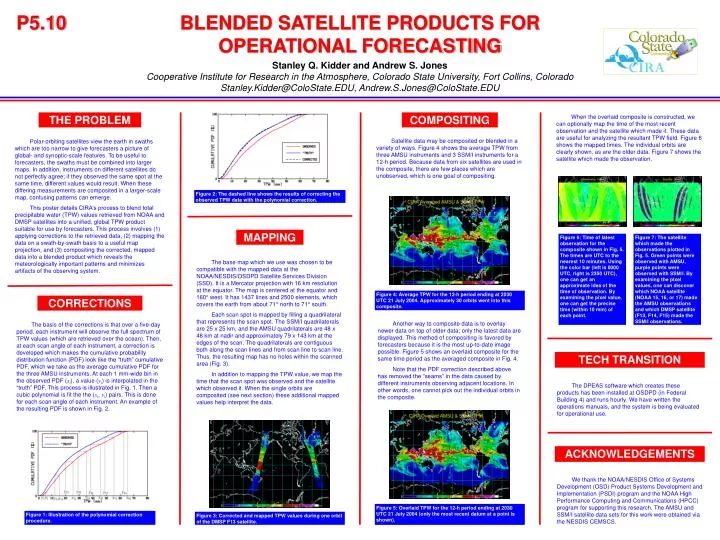
1. THE PROBLEM COMPOSITING When the overlaid composite is constructed, we can optionally map the time of the most recent observation and the satellite which made it. These data are useful for analyzing the resultant TPW field. Figure 6 shows the mapped times. The individual orbits are clearly shown, as are the older data. Figure 7 shows the satellite which made the observation. Satellite data may be composited or blended in a variety of ways. Figure 4 shows the average TPW from three AMSU instruments and 3 SSM/I instruments for a 12-h period. Because data from six satellites are used in the composite, there are few places which are unobserved, which is one goal of compositing. Polar-orbiting satellites view the earth in swaths which are too narrow to give forecasters a picture of global- and synoptic-scale features. To be useful to forecasters, the swaths must be combined into larger maps. In addition, instruments on different satellites do not perfectly agree; if they observed the same spot at the same time, different values would result. When these differing measurements are composited in a larger-scale map, confusing patterns can emerge. This poster details CIRA’s process to blend total precipitable water (TPW) values retrieved from NOAA and DMSP satellites into a unified, global TPW product suitable for use by forecasters. This process involves (1) applying corrections to the retrieved data, (2) mapping the data on a swath-by-swath basis to a useful map projection, and (3) compositing the corrected, mapped data into a blended product which reveals the meteorologically important patterns and minimizes artifacts of the observing system. Figure 2: The dashed line shows the results of correcting the observed TPW data with the polynomial correction. Figure 6: Time of latest observation for the composite shown in Fig. 5. The times are UTC to the nearest 10 minutes. Using the color bar (left is 0000 UTC, right is 2350 UTC), one can get an approximate idea of the time of observation. By examining the pixel value, one can get the precise time (within 10 min) of each point. Figure 7: The satellite which made the observations plotted in Fig. 5. Green points were observed with AMSU, purple points were observed with SSM/I. By examining the pixel values, one can discover which NOAA satellite (NOAA 15, 16, or 17) made the AMSU observations and which DMSP satellite (F13, F14, F15) made the SSM/I observations. MAPPING The base map which we use was chosen to be compatible with the mapped data at the NOAA/NESDIS/OSDPD Satellite Services Division (SSD). It is a Mercator projection with 16 km resolution at the equator. The map is centered at the equator and 160° west. It has 1437 lines and 2500 elements, which covers the earth from about 71° north to 71° south. Each scan spot is mapped by filling a quadrilateral that represents the scan spot. The SSM/I quadrilaterals are 25 x 25 km, and the AMSU quadrilaterals are 48 x 48 km at nadir and approximately 79 x 143 km at the edges of the scan. The quadrilaterals are contiguous both along the scan lines and from scan line to scan line. Thus, the resulting map has no holes within the scanned area (Fig. 3). In addition to mapping the TPW value, we map the time that the scan spot was observed and the satellite which observed it. When the single orbits are composited (see next section) these additional mapped values help interpret the data. Figure 4: Average TPW for the 12-h period ending at 2030 UTC 21 July 2004. Approximately 30 orbits went into this composite. CORRECTIONS Another way to composite data is to overlay newer data on top of older data; only the latest data are displayed. This method of compositing is favored by forecasters because it is the most up-to-date image possible. Figure 5 shows an overlaid composite for the same time period as the averaged composite in Fig. 4. Note that the PDF correction described above has removed the “seams” in the data caused by different instruments observing adjacent locations. In other words, one cannot pick out the individual orbits in the composite. The basis of the corrections is that over a five-day period, each instrument will observe the full spectrum of TPW values (which are retrieved over the ocean). Then, at each scan angle of each instrument, a correction is developed which makes the cumulative probability distribution function (PDF) look like the “truth” cumulative PDF, which we take as the average cumulative PDF for the three AMSU instruments. At each 1 mm-wide bin in the observed PDF (xi), a value (yi) is interpolated in the “truth” PDF. This process is illustrated in Fig. 1. Then a cubic polynomial is fit the the (xi, yi) pairs. This is done for each scan angle of each instrument. An example of the resulting PDF is shown in Fig. 2. TECH TRANSITION The DPEAS software which creates these products has been installed at OSDPD (in Federal Building 4) and runs hourly. We have written the operations manuals, and the system is being evaluated for operational use. ACKNOWLEDGEMENTS We thank the NOAA/NESDIS Office of Systems Development (OSD) Product Systems Development and Implementation (PSDI) program and the NOAA High Performance Computing and Communications (HPCC) program for supporting this research. The AMSU and SSM/I satellite data sets for this work were obtained via the NESDIS CEMSCS. Figure 5: Overlaid TPW for the 12-h period ending at 2030 UTC 21 July 2004 (only the most recent datum at a point is shown). Figure 3: Corrected and mapped TPW values during one orbit of the DMSP F13 satellite. Figure 1: Illustration of the polynomial correction procedure. P5.10 BLENDED SATELLITE PRODUCTS FOR OPERATIONAL FORECASTING Stanley Q. Kidder and Andrew S. Jones Cooperative Institute for Research in the Atmosphere, Colorado State University, Fort Collins, Colorado Stanley.Kidder@ColoState.EDU, Andrew.S.Jones@ColoState.EDU