Download
1 / 23
230 likes | 368 Views
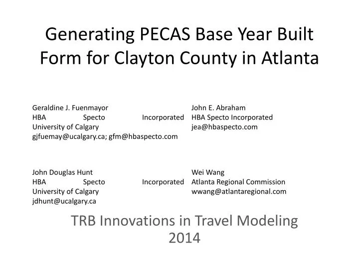
Generating PECAS Base Year Built Form for Clayton County in Atlanta. TRB Innovations in Travel Modeling 2014. Context. PECAS Spatial Economic and Land Use Model for Atlanta Constructed and calibrated being used for policy analysis and forecasting ( incl RTP)

E N D
Generating PECAS Base Year Built Form for Clayton County in Atlanta TRB Innovations in Travel Modeling 2014
Context • PECAS Spatial Economic and Land Use Model for Atlanta • Constructed and calibrated • being used for policy analysis and forecasting (incl RTP) • “Agile and Incremental Project Management” • Production-ready model • and ongoing improvements • One type of ongoing improvement is replacing information on base-year built-form • And previous Clayton County data was quite bad
Economy size forecast (REMI) Economy size forecast (REMI) Transport demand model Transport demand model PECAS Economic Conditions EconomySize EconomySize SpaceInventory SD - Space Development Module AA - Economic Interactions Module AA - Economic Interactions Module Rents Locations/Interactions Locations/Interactions Travel Conditions Time t + 1 Time t
Issues with land use data • Spatial consumptions rates heterogeneous and elastic • Even within the most detailed industrial classifications • Measurement errors in both employment and building data • Across the word, and even in the USA • Categorical mismatch in built form descriptions
Employment and floorspace calibration elasticities/ substitutions Floorspace consumption rates Employment Population Locations Measured Quantity of Space by TAZ Modeled Quantity of Space by LUZ Activity Allocation Module Observed Space Rents Modeled Space Rents Input Output Economic Relationships Transport Costs (willingness to travel to interact)
Options for SD Base Year Parcel Database • Option 1: SD uses observed parcel data, even thought it has obvious mistakes and is not compatible with AA’s view of the world. • Difference stored in “FloorspaceDelta” file. • Option NAO: Spend the rest of your life trying to “fix the parcel data” • Option 2: Develop a Synthetic Parcel Database that respects the measured data as much as possible, but is consistent with simplified model and the tradeoffs made in calibration.
FI - Floorspace inventory PG - Parcel Geodatabase changing columns during FS assignment FS - Floorspace Synthesizer Output shape file (Initial runs) Scoring System: Level 1: assign a score from match column MCT - Match Coefficient Table Calibration Strategies and adjustments Output shape file (Calibrated Targets) Level 2: score – penalty function (FAR) Level 3: final penalty (based on space)
FI - Floorspace inventory PG - Parcel Geodatabase changing columns during FS assignment Figure 2. Floorspace Synthesizer: Floorspace Inventory and Parcel Geodatabase
FS - Floorspace Synthesizer Output shape file (Initial runs) Scoring System: Level 1: assign a score from match column MCT - Match Coefficient Table Figure 3. Floorspace Synthesizer Scoring System, Output Files, Calibration Strategies and Calibrated Targets Calibration Strategies and adjustments Output shape file (Calibrated Targets) Level 2: score – penalty function (FAR) Level 3: final penalty (based on space)
Penalty when FAR gets too high Score Look up attributes for suitability Penalty and bonus for already assigned space
The synthesizer was correct in assigning residential space to parcels that had been observed to have agriculture land; but it had no information to identify which of the “observed agricultural” parcels it should use Figure 4. Example of parcels with agriculture assigned as single family
Implications / Conclusions • Data are wrong • And when they are right, are inconsistent in other ways • Theory helps identify inconsistencies • Strong theoretical model also needs system for dealing with inconsistencies • Incremental model data improvement program
Implications / Conclusions • Scoring system identified best possible parcels to hold compromise space quantity • Scores based on observed parcel attributes • Comparing assigned vs observed type/intensity showed TAZ level inconsistencies. • Tracked to incorrect/suspect data and odd places like airports • Correct problems, accept inconsistencies, or modify scoring to put buildings in better locations