Download
1 / 58
580 likes | 612 Views
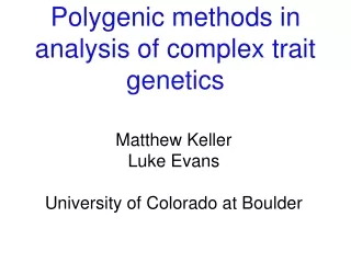
Polygenic methods in analysis of complex trait genetics. Matthew Keller Luke Evans University of Colorado at Boulder. Polygenicity in complex traits. The sum of R 2 of significantly associated SNPs of complex traits typically < 10%, despite twin/family h 2 ~ .5 +/-.2. Why ?

E N D
Polygenic methods in analysis of complex trait genetics Matthew Keller Luke Evans University of Colorado at Boulder
Polygenicity in complex traits • The sum of R2 of significantly associated SNPs of complex traits typically < 10%, despite twin/family h2 ~ .5 +/-.2. Why? • One possibility: large number of small-effect (~ the 'infinitesimal model'; Fisher, 1918) causal variants (CVs) that failed to reach genome-wide significance (many type-II errors) • Growing consensus: 100s to 1000s of CVs contribute to the genetic variation of traits like schizophrenia, each with small effects (OR < 1.3), often in unpredicted loci
Should we continue to do candidate gene research on complex traits?
Should we continue to do candidate gene research on complex traits? NO
Outline • Estimating prediction accuracy of polygenic risk scores (PRS) from GWAS • history • how it works • interpretations, uses, & pitfalls • Estimating VA explained by all SNPs using genetic similarity at SNPs • how it works - HE-regression example • walk through of GREML approach • practical issues – SNP & individual QC
Outline • Estimating prediction accuracy of polygenic risk scores (PRS) from GWAS • history • how it works • interpretations, uses, & pitfalls • Estimating VA explained by all SNPs using genetic similarity at SNPs • how it works - HE-regression example • walk through of GREML approach • practical issues – SNP & individual QC
History of PRS • In the dark ages of complex trait genetics (04-09), many geneticists had lost all hope of finding a way to get their N=3k GWAS samples published.
History of PRS • In the dark ages of complex trait genetics (04-09), many geneticists had lost all hope of finding a way to get their N=3k GWAS samples published. • Then, in 2009, a giant in our field, Sean Purcell, decided to look at the conglomerate effects of thousands of SNPs on a trait and found signals. The floodgates opened.
History of PRS Polygenic Risk Score (PRS) – aka – the “Purcell” approach
History of PRS Polygenic Risk Score (PRS) – aka – the “Purcell” approach
History of PRS Polygenic Risk Score (PRS) – aka – the “Purcell” approach aka – the David Evans Polygenic Risk Score Ingenious (DEPRSING) Approach
Polygenic Risk Score (PRS) Steps • Obtain GWAS summary statistics (p-values and β’s) in largest possible discovery sample • Obtain independent target sample with genomewide data • Use SNPs in common between the two samples. • (Optional) Deal with association redundancy due to LD. • Restrict to SNPs with p < various thresholds (1e-5,1e-4…0.5...1.0). • Construct PRS = sum of risk alleles weighted by β from regression. • Regress trait in target sample onto PRS. Evaluate strength of this association (r2 or h2 in liability threshold model).
Step 1–GWAS in discovery sample Psychiatric Genomics Consortium, Nature, 2014
Polygenic Risk Score (PRS) Steps • Obtain GWAS summary statistics (p-values and β’s) in largest possible discovery sample • Obtain independent target sample with genomewide data • Use SNPs in common between the two samples. • (Optional) Deal with association redundancy due to LD. • Restrict to SNPs with p < various thresholds (1e-5,1e-4…0.5...1.0). • Construct PRS = sum of risk alleles weighted by β from regression. • Regress trait in target sample onto PRS. Evaluate strength of this association (r2 or h2 in liability threshold model).
Step 2 – Crucial: target & discovery samples are independent • If non-independence between discovery & target, r2target will be overestimated • If some of the same people are in both • If there are close relatives between the two • If you preselect most significant SNPs in target + discovery sample first, then follow the normal PRS procedures
Why non-independence inflates r2 • If null true, E(r2discovery) ≅ 1/N. (This is also E[r2target] if no PRS association) • m unassociated, uncorrelated SNPs, E(r2discovery) ≅ m/N • If choose the m most associated SNPs of 100K, the problem is even worse.
Why non-independence inflates r2 • If null true, E(r2discovery) ≅ 1/N. (This is also E[r2target] if no PRS association) • m unassociated, uncorrelated SNPs, E(r2discovery) ≅ m/N • If choose the m most associated SNPs of 100K, the problem is even worse. • E(r2discovery) = Wray et al, 2013. Pitfalls of predicting complex traits from SNPs.
Why non-independence inflates r2 • If null true, E(r2discovery) ≅ 1/N. (This is also E[r2target] if no PRS association) • m unassociated, uncorrelated SNPs, E(r2discovery) ≅ m/N • If choose the m most associated SNPs of 100K, the problem is even worse. • E.g., Ndiscovery=10k. E(r2discovery) ≅ .10 if choose m=1k randomly, but E(r2discovery) ≅ .60 if choose m=1k biggest
Why non-independence inflates r2 • If null true, E(r2discovery) ≅ 1/N. (This is also E[r2target] if no PRS association) • m unassociated, uncorrelated SNPs, E(r2discovery) ≅ m/N • If choose the m most associated SNPs of 100K, the problem is even worse. • E.g., Ndiscovery=10k. E(r2discovery) ≅ .10 if choose m=1k randomly, but E(r2discovery) ≅ .60 if choose m=1k biggest • If q proportion of target sample that overlaps, E(r2) in that part of sample is same as in discovery sample. Thus under null: • E(r2target) ≅ q*r2discovery + (1-q)*1/Ntarget
Polygenic Risk Score (PRS) Steps • Obtain GWAS summary statistics (p-values and β’s) in largest possible discovery sample • Obtain independent target sample with genomewide data • Use SNPs in common between the two samples. • (Optional) Deal with association redundancy due to LD. • Restrict to SNPs with p < various thresholds (1e-5,1e-4…0.5...1.0). • Construct PRS = sum of risk alleles weighted by β from regression. • Regress trait in target sample onto PRS. Evaluate strength of this association (r2 or h2 in liability threshold model).
Step 3 – Use SNPs in common Array Data Imputed Data Affy Axiom Illumina 1M If discovery & target on different arrays, use imputed data to maximize overlap
Polygenic Risk Score (PRS) Steps • Obtain GWAS summary statistics (p-values and β’s) in largest possible discovery sample • Obtain independent target sample with genomewide data • Use SNPs in common between the two samples. • (Optional) Deal with association redundancy due to LD. • Restrict to SNPs with p < various thresholds (1e-5,1e-4…0.5...1.0). • Construct PRS = sum of risk alleles weighted by β from regression. • Regress trait in target sample onto PRS. Evaluate strength of this association (r2 or h2 in liability threshold model).
Step 4 – Account for LD • CVs inflate associations of nearby SNPs they are in LD with redundant signals. Thus: • r2target depends strongly on distribution of SNPs • Diminishes genomewide signal interpretation • Typically, people account for LD (worst to best): • LD prune – but can lose strongest signals • LD clumping – preferentially leave in strongest signals, prune out weaker ones in LD • Model LD – LDpred (Vihjalmsson et al, AJHG, 2015)
Polygenic Risk Score (PRS) Steps • Obtain GWAS summary statistics (p-values and β’s) in largest possible discovery sample • Obtain independent target sample with genomewide data • Use SNPs in common between the two samples. • (Optional) Deal with association redundancy due to LD. • Restrict to SNPs with p < various thresholds (1e-5,1e-4…0.5...1.0). • Construct PRS = sum of risk alleles weighted by β from regression. • Regress trait in target sample onto PRS. Evaluate strength of this association (r2 or h2 in liability threshold model).
Step 5 – Use various p thresholds Use p-thresholds from 5e-8,1e-7,…0.5...0. Report results from all thresholds
Polygenic Risk Score (PRS) Steps • Obtain GWAS summary statistics (p-values and β’s) in largest possible discovery sample • Obtain independent target sample with genomewide data • Use SNPs in common between the two samples. • (Optional) Deal with association redundancy due to LD. • Restrict to SNPs with p < various thresholds (1e-5,1e-4…0.5...1.0). • Construct PRS = sum of risk alleles weighted by β from regression. • Regress trait in target sample onto PRS. Evaluate strength of this association (r2 or h2 in liability threshold model).
Step 6: Construct PRS • PRSj = Σ [βi,discovery * SNPij] • βi,discovery = effect size in discovery sample from OLS (continuous trait) or logistic reg (binary trait; β = log(OR)) • SNPij = # alleles (0,1,2) for SNP i of person j in target sample • In PLINK, --score.
Polygenic Risk Score (PRS) Steps • Obtain GWAS summary statistics (p-values and β’s) in largest possible discovery sample • Obtain independent target sample with genomewide data • Use SNPs in common between the two samples. • (Optional) Deal with association redundancy due to LD. • Restrict to SNPs with p < various thresholds (1e-5,1e-4…0.5...1.0). • Construct PRS = sum of risk alleles weighted by β from regression. • Regress trait in target sample onto PRS. Evaluate strength of this association (r2 or h2 in liability threshold model).
Step 7: Evaluation of PRS • For continuous traits, this is simply the r2 from an OLS regressing continuous trait ~ PRS in target. • Trickier for binary (e.g., case-control) data. • Nagelkerke’s R2 often used. But it has unfortunate property of depending on disease prevalence & proportion of cases: Wray et al, 2013. Pitfalls of predicting complex traits from SNPs.
Step 7: Evaluation of PRS • For continuous traits, this is simply the r2 from an OLS regressing continuous trait ~ PRS in target. • Trickier for binary (e.g., case-control) data. • Nagelkerke’s R2 often used. But it has unfortunate property of depending on disease prevalence & proportion of cases. • Not comparable to h2 as usually estimated • Better alternative = h2 on the liability scale§, which can be found by converting r2 from an OLS regression of binary trait ~ PRS to h2. • §see Lee et el., 2012. Genetic Epidemiology. A better coefficient of determination for genetic profile analysis.
Interpretation of r2 from PRS • r2target is an estimate of how well one can predict a trait. But prediction accuracy is lower than estimation accuracy. • Variance of PRS is a sum of two components per SNP: • true component – often 0 or close to 0 • error component ≅ V(SNP) * V(Y)/[2*p*q*N] = V(Y)/N • Unless N very large (e.g., millions), error swamps true component, and PRS is mostly noise. • Thus, PRS r2 is a (typically severely) downwardly biased estimate of SNP-h2 • As N ∞, PRS r2SNP-h2
Power & accuracy of PRS’s • Ndiscovery E[r2target]Ntarget no influence E[r2target] • Ndiscovery power[r2target]Ntarget power[r2target] • For large Ndiscovery (>>10k), typically sufficient power to detect PRS relationship at α=.05 with Ntarget >1k. • Optimal split of Ndiscovery vs. Ntarget: • To maximize power, split discovery & target equally • To maximize prediction accuracy, maximize Ndiscovery Dudbridge (2013). PLoS Gen. Power and predictive accuracy of polygenic risk scores
Outline • Estimating prediction accuracy of polygenic risk scores (PRS) from GWAS • history • how it works • interpretations, uses, & pitfalls • Estimating VA explained by all SNPs using genetic similarity at SNPs • how it works - HE-regression example • walk through of GREML approach • practical issues – SNP & individual QC
Using genetic similarity at SNPs to estimate VA • Determine extent to which genetic similarity at SNPs is related to phenotypic similarity • Multiple approaches to derive unbiased estimate of VA captured by measured (common) SNPs • Regression (Haseman-Elston) • Mixed effects models (GREML) • Bayesian (e.g., Bayes-R) • LD-score regression
Regression estimates of h2 product of centered scores (here, z-scores) (the slope of the regression is an estimate of h2)
Regression estimates of h2 (the slope of the regression is an estimate of h2)
Regression estimates of h2 COR(MZ) (the slope of the regression is an estimate of h2)
Regression estimates of h2 COR(DZ) (the slope of the regression is an estimate of h2)
Regression estimates of h2 2*[COR(MZ)-COR(DZ)]= h2 = slope (the slope of the regression is an estimate of h2)
Regression estimates of h2 (the slope of the regression is an estimate of h2)
Regression estimates of h2 (the slope of the regression is an estimate of h2)
Regression estimates of h2snp (the slope of the regression is an estimate of h2)
Interpreting h2 estimated from SNPs (h2snp) • If close relatives included (e.g., sibs), h2snp≅ h2 estimated from a family-based method, because great influence of extreme pihats. Interpret h2snp as from these designs. • If use ‘unrelateds’(e.g., pihat < .05): • h2snp = proportion of VP due to VA captured by SNPs. Upper bound % VP GWAS can detect • Gives idea of the aggregate importance of CVs tagged by SNPs • By not using relatives who also share environmental effects: (a) VA estimate 'uncontaminated' by VC & VNA; (b) does not rely on family study assumptions (e.g., r(MZ) > r(DZ) for only genetic reasons)
GREML Model (here, n=3, q=2 fixed effects, m=3 SNPs) n×m 1.15 -.58 -1.15 -.58 1.15 .58 -.58 -.58 .58 3 -5 2 • -1.2 • 1 0.8 • 0.4 * * + + = design matrix for SNP effects = design matrix of fixed effects (intercept & 1 covariate) observed y fixed effects residuals SNP effects