SPH simulations of star formation triggered by expanding HII regions

1. SPH simulations of star formation triggered by expanding HII regions Thomas G. Bisbas Cardiff University Collaborators: Anthony Whitworth, Richard Wünsch, David Hubber and Stefanie Walch. Prague, 16th September 2009. CONSTELLATION meeting.

2. Outline • Radiation Driven Compression • Numerical treatment and transport of ionizing photons • Description of the simulations • Results • Conclusions

3. Radiation Driven Compression

4. Radiation Driven Compression The structure of the interstellar medium is observed to be extremely irregular and to contain many clouds. As an HII region expands, it may overrun and compress pre-existing nearby clouds, causingthemto collapse. As they collapse, their internal thermal pressure increases and this leads to re-expansion. After re-expansion, a cometary tail is formed extending away from the ionizing source. The above process is known as Radiation Driven Compression (or Implosion). Lefloch & Lazareff (1994)

5. Radiation Driven Compression If the head of this cometary structure is too dense, it fragments. These globules are therefore potential sites of star formation. Various observations show the existence of these structures (Sugitani et al. 1999; Lefloch & Lazareff 1995; Lefloch et al. 1997; Morgan et al. 2008; and others). Several workers have tried to simulate the Radiation Driven Compression process. Some of these simulations concentrate on the morphology of the resulting bright-rimmed clouds (Sandford et al. 1982; Bertoldi 1989; Lefloch & Lazareff 1994; Miao et al. 2006; Henney et al. 2008), and some others explore the possibility that the collapse of a bright-rimmed cloud might sometimes lead to triggered star formation (Kessel-Deynet & Burkert 2003; Dale et al. 2005; Miao et al. 2008; Gritschneder et al. 2009). However, as Deharveng et al. (2005) mention, “no model explains where star formation takes place (in the core or at its periphery) or when (during the maximum compression phase, or earlier).”

6. Numerical treatment and transport of ionizing photons

7. Numerical treatment and transport of ionizing photons y RIF The D – type expansion of an HII region y x The ionization front (IF) is located where x where m = mp / X. In the simulations presented here we use X=0.7 which corresponds to H2 The integral which we want to solve is: Stromgren Sphere Neutral cloud

8. Numerical treatment and transport of ionizing photons Ray Casting We use SEREN SPH code (Hubber et al. 2009, in preparation). We use HEALPix algorithm (Gorski et al. 2005) to generate a uniform set of rays, in order to determine the overall shape of the ionization front. where is the level of refinement How many rays? Gorski et al. (1999)

9. Numerical treatment and transport of ionizing photons Ray Casting To perform the integration we define a set of discrete evaluation points. The SPH density at each point is We use the trapezium method of integration to calculate the integral I. Acceptable accuracy is obtained with f1=0.25 The next evaluation point is f1hj’ * j’+1 j’ j’-1 Source

10. Numerical treatment and transport of ionizing photons Ray Splitting A ray is split into four child-rays as soon as its linear separation from the neighbouring rays exceeds f2hj Acceptable accuracy is obtained with f2=0.5 Abel & Wandelt (2002)

11. Numerical treatment and transport of ionizing photons Ray Splitting Family Ray Ionizing source Ionization Front Ray at level l-1 Ray at level l Ray at level l+1 Child-ray Mother-ray

12. Numerical treatment and transport of ionizing photons Ray Splitting Family Ray Ionizing source Ionization Front Ray at level l-1 Ray at level l Ray at level l+1 Child-ray Mother-ray

13. Numerical treatment and transport of ionizing photons Ray Splitting Family Ray Ionizing source Ionization Front Ray at level l-1 Ray at level l Ray at level l+1 Child-ray Mother-ray

14. Numerical treatment and transport of ionizing photons Ray Splitting Family Ray Ionizing source Ionization Front Ray at level l-1 Ray at level l Ray at level l+1 Child-ray Mother-ray

15. Numerical treatment and transport of ionizing photons Ray Splitting Family Ray Ionizing source Ionization Front Ray at level l-1 Ray at level l Ray at level l+1 Child-ray Mother-ray

16. Numerical treatment and transport of ionizing photons Bisbas et al. (2009)

17. Description of the simulations

18. Description of the simulations Bonnor-Ebert sphere The dimensionless radius ξB is where RB is the radius of the sphere, RC is the radius of the core which reads and ρC is the density at the centre of the sphere. Stability analysis show that for ξB < 6.451 the sphere is stable and for ξB > 6.451 it is unstable. ρ ρC We use stable Bonnor-Ebert spheres with ξB = 4 ρB RC RB r

19. Description of the simulations We use a barotropic equation of state of the form where is the thermal pressure of the gas is the density of the gas is the critical density is the sound speed for is the ratio of specific heats The temperature of the gas is where is the temperature of the gas at low densities

20. y R D x Description of the simulations We introduce the dimensionless parameter and we run simulations for λ=2, 5, 10.

21. Description of the simulations We define here the terminology that we will use in our discussion. We call: Star Formation (SF): when the clump during the compression becomes gravitationally unstable and forms stars Acceleration (A): when the clump does not become gravitationally unstable during the compression and it simply re-expands and evaporates Evaporation (E): when the incident flux is so strong that it fully evaporates it instantly

22. Description of the simulations Technical tests We perform technical tests in order to explore the capabilities of our code in modeling star formation in clumps ionized by an external source. In particular, we examine how the physical quantities of Bonnor-Ebert spheres, such as their morphological evolution and their star formation efficiency, are affected by the numerical noise of the calculations. To do this, we consider the 2Mo Bonnor-Ebert sphere with λ=2 (R=0.12, D=0.24pc). We run 4 simulations were we perturb very little the initial positions of this sphere.

24. Description of the simulations • Results of technical tests • The sink creation time, , remains unchanged. • The neutral remaining mass, at remains unchanged. • The total number of sink particles formed, , strongly depends on the numerical noise. • The total mass of sink particles formed, , is quite similar in all four simulations.

25. Results

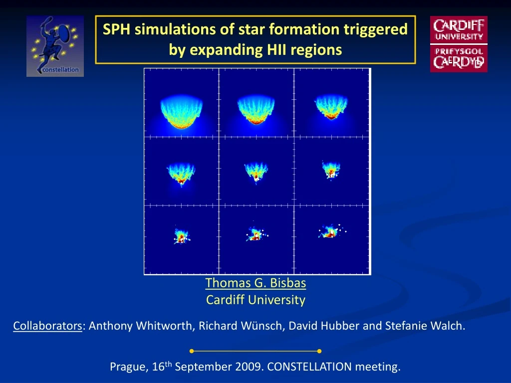
26. Results The curvature of the incident flux delays fragmentation Since we place the Bonnor-Ebert spheres at various distances from the source, it is interesting to see how the curvature of the incident flux affects their evolution. To do this we perform a set of three simulations where we place the 2Mo at various distances D in order to have λ=2,5,10, and we keep constant the incident flux ΦD = 1.45 x 1011 cm-2s-1.

27. Results The curvature of the incident flux delays fragmentation λ=2 λ=10 λ=10 λ=5 Observe that the surface density of the shocked core is lower for lower λ, and therefore the gravitational forces in the layer are weaker. In addition, the shocked material has a greater tangential divergence for lower λ. Both these factors act to delay fragmentation, and hence also sink creation, when is small. λ=2

28. Results

29. Snapshots were taken at sink creation time, Results M = 2 Mo M = 10 Mo M = 5 Mo

31. Results The flux-mass diagram Semi-logarithmic diagram where we define the zones `Star Formation', `Acceleration', and `Evaporation’. The logarithmic x-axis of this diagram is the incident flux (log Φ) and the y-axis is the initial mass M of the clump. From these simulations it is not possible to define the exact location for the transition of one zone to another. However, it is clear that as the mass M of these Bonnor-Ebert spheres decreases, they appear to survive more in higher fluxes.

32. A common feature amongst the morphological structures at sink creation time, is that stars form along the line of sight towards the exciting star (agreement with Sugitani et al. 1999) We define as the distance of the first sink particle formed from the ionization front. We plot versus Φ. We omit the simulations with the irregular jelly-fish structu-re. Results Stars form close to the periphery with increasing the flux M = 2 Mo

33. Results Stars form close to the periphery with increasing the flux The first zone (1) corresponds to low fluxes. Here, stars tend to form along the filamentary structure and particularly at its innermost part. The second zone (2) corresponds to intermediate fluxes. Here, the filament becomes smaller and therefore stars tend to form closer to the periphery. Finally, the third zone (3) corresponds to high fluxes. The filamentary structure here cannot be developed and therefore stars are formed at the periphery.

34. We define as the width of the two sides of each clump and we normalize it with the initial radius of each Bonnor-Ebert sphere, . This value represents the measure of compression. We plot versus the incident flux Φ. We omit the simulations with the irregular jelly-fish structu-re. Results Stars form during maximum compression with increasing the flux M = 2 Mo

35. Results Stars form during maximum compression with increasing the flux Compression is a result of: Zone 1: Ionization + Gravity Zone 2: Ionization only 1 2

36. Results Low fluxes increase the total mass of stars Zone 1: Stars formed at the innermost regions. Compression is supported by ionization and mutual gravity. Low fluxes favour the total final mass of the sink particles. Zone 2: Stars tend to form closer to the periphery. Compression is supported by ionization only. Intermediate fluxes form stars with total mass about 30% of the initial mass of the clumps. Zone 3: Stars formed at the periphery. Compression is supported by ionization only. High fluxes act to form stars with low total mass.

37. Conclusions

38. Conclusions We examined clumps of various masses and fluxes of various intensities. In general we find a connection between the incident flux and the corresponding star formation efficiency. We propose a flux-mass diagram to map the resultant production of each simulation. Our results can be summarized as follows: Low fluxes: An extended filamentary structure develops. Stars tend to form at its innermost part. The filament increases the mutual gravitational forces of the initial clump which increase its compression. The total final mass of stars is high comparing with the initial mass of the clump. Intermediate fluxes: The filamentary structure is small. Morphology is close to U-shape. Stars tend to form closer to the periphery. Ionization starts to be the dominant factor of compressing the initial clump. The total final mass of stars is about 30% of the initial mass of the clump. High fluxes: No filamentary structure. Morphology is close to V-shape. Stars form at the periphery. Ionization is the dominant factor of compression. The total final mass of stars is very low. Very high fluxes: No star formation. The clumps are being accelerated and evaporated.

39. References Abel, T., & Wandelt, B.D. 2002, MNRAS, 330, L53 Bertoldi, F. 1989, ApJ, 346, 735 Bisbas, T. G., Wunsch, R., Whitworth, A. P., & Hubber, D. A., 2009, A&A, 497, 649 Dale, J.E., Bonnell, I. A., Clarke, C. J., & Bate, M. R. 2005, MNRAS, 358, 291 Deharveng, L., Zavagno, A., & Caplan, J. 2005, A&A, 433, 565 Gorski, K. M., Hivon, E., Banday, A. J., Wandelt, B. D., Hansen, F. K., et al. 2005, ApJ, 622, 759 Gritschneder, M., Naab, T., Burkert, A., Walch, S., Heitsch, F., & Wertzstein, M. 2009, MNRAS, 339, 21 Henney, W. J., Arthur, S. J., De Colle, F., & Mellema, G. 2009, MNRAS, 398, 157 Hubber et al. 2009, in preparation Kessel-Deynet, O., & Burkert, A. 2003, MNRAS, 338, 545 Lefloch, B., & Lazareff, B. 1994, A&A, 289, 559 Lefloch, B., & Lazareff, B. 1995, A&A, 301, 522 Lefloch, B., Lazareff, B., & Castets, A. 1997, A&A, 324, 249 Miao, J., White, G. J., Nelson, R., Thompson, M., & Morgan, L. 2006, MNRAS, 369, 143 Miao, J., White, G. J., Thompson, M. A., & Nelson, R. P. 2009, ApJ, 692, 382 Morgan, L. K., Thompson, M. A., Urquhart, J. S., & White, G. J. 2008, A&A, 477, 577 Price, D.J. 2007, Publications of the Astronomical Society of Australia, 24, 159 Sandford, M. T., II, Whitaker, R. W., & Klein, R. I. 1982, ApJ, 260, 183 Sugitani, K., Tamura, M., & Ohura, K. 1999, Star Formation 1999, Proceedings of Star Formation 1999, held in Nagoya, Japan, June 21-25, 1999, Editor: T. Nakamoto, Nobeyama Radio Observatory, p. 358-364, 358.

40. EXTRA SLIDES BEYOND THIS POINT

41. Profile of the simulations Uniform density Bonnor-Ebert sphere ρ ρ r r

42. Radiation Driven Compression Lefloch & Lazareff test Bisbas et al. (2009) Lefloch & Lazareff (1994)