SKTN 2393 Numerical Methods for Nuclear Engineers

1. SKTN 2393 Numerical Methods for Nuclear Engineers Chapter 7 Numerical Integration MohsinMohdSies Nuclear Engineering, School of Chemical and Energy Engineering, UniversitiTeknologi Malaysia

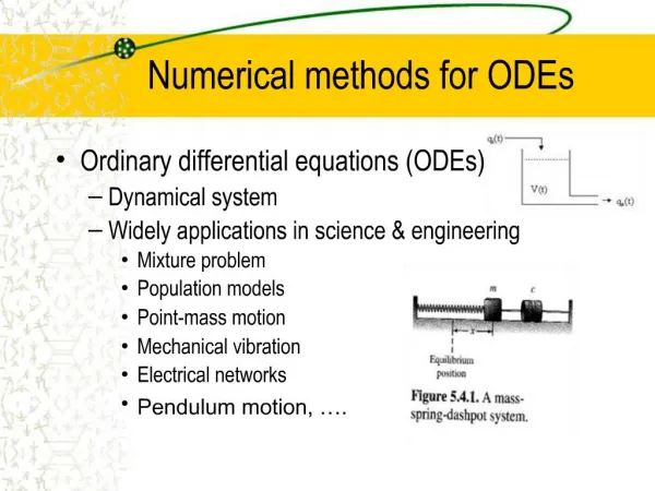
2. Introduction Many engineering problems require the evaluation of the integral where f (x) is integrand and a and b are limits of integration. One of the major use of integral calculus was the calculation of areas and volumes of irregularly shaped region. If f (x) is continuous, finite and well behaved over the range of integration , integral I can be evaluated analytically

3. Introduction • Numerical integration, a.k.a. numerical quadrature, is an approximation of definite integrals and used in cases where • f(x) is a complicated continuous function that is difficult or impossible to integrate in closed form • f(x) is in tabular form, where values of x and f(x) are available at a number of discrete point in range • limits of integration may be infinite • f(x) may be discontinuous or may become infinite at some point in range

4. Introduction Integral of function f (x) between limits a and b denotes the area under the curve of f (x) between limits a and b

5. Introduction • Functions to be integrated numerically are in two forms: • A table of values. We are limited by the number of points that are given. • A function. We can generate as many values of f(x) as needed to attain acceptable accuracy.

6. Sample Engineering Problems Problem Statement: The variation of torque of an engine with the angular displacement of the crank is shown in Table 1. Use a graphical method to determine the energy generated during a cycle by integrating the torque-displacement function over a cycle. Hint: Work = (Torque)× (Angular displacement)

8. Sample Engineering Problems

9. Sample Engineering Problems

10. Methods Available • Newton-Cotes Quadrature • Rectangular Rule • Trapezoidal Rule • Simpson’s 1/3 Rule • Simpson’s 3/8 Rule • Gauss Quadrature • Gauss-Legendre Formula • Gauss-Chebyshev Formula • Gauss-Hermite Formula

11. Newton-Cotes Integration Formulas • The Newton-Cotes formulas are the most common numerical integration schemes. • They are based on the strategy of replacing a complicated function or tabulated data with an approximating function that is easy to integrate: • A polynomial of order n is the preferred approximating function since it is easy to integrate.

12. Approximating Functions

13. Approximating Functions

14. Newton-Cotes - Multiple Application • The function or data of f (x) can also be approximated using a series of piecewise polynomials, also called the multiple application. • Range of integration, , is divided into a finite number, n, of equal intervals. Width of each interval is • Discrete points or nodes in the range of integration is given by

15. Newton-Cotes - Multiple Application

16. Rectangular Rule If values of f (x) is approximated by its values at the beginning of each interval, the area under the curve f (x) in the interval is taken as and the integral I is evaluated as If values of f (x) is approximated by its values at the end of each interval, the area under the curve f (x) in the interval is taken as and the integral I is evaluated as

17. Rectangular Rule Under- and over-estimation of integral I

18. Rectangular Rule – Midpoint Method An improvement in accuracy of the piecewise-constant approximation can be achieved by using the average value of and in the interval . The integral is now evaluated as

19. Rectangular Rule Choosing interval h that is too large can lead to very large errors

20. Trapezoidal Rule • Extensively used in engineering applications. Simplicity in developing computer program. • Applies for equally spaced base points only • Approximation of f (x) by piecewise polynomial of order one which is a straight line • Area under the curve is equal to the area of the trapezoid, thus the name

21. Trapezoidal Rule • The Trapezoidal rule is the first of the Newton-Cotes closed integration formulas, corresponding to the case where the polynomial is first order: • The area under this first order polynomial is an estimate of the integral of f(x) between the limits of a and b: Trapezoidal rule

22. Trapezoidal Rule – Multiple Application • One way to improve the accuracy of the trapezoidal rule is to divide the integration interval from a to b into a number of segments and apply the method to each segment. • The areas of individual segments can then be added to yield the integral for the entire interval. • Substituting the trapezoidal rule for each interval yields where h is the (equally spaced) increment between two adjacent nodes.

23. Example f(x) = 0.84885406 + 31.51924706x − 137.66731262x^2 + 240.55831238x^3 − 171.45245361x^4+ 41.95066071x^5

24. Simpson’s Rules • Accuracy of the trapezoidal rule can be improved by increasing the number of segments n or reducing step size h; but this eventually leads to increase in round-off error. • Another way to get more accurate estimate of integral is to use higher order polynomials for approximating the function f (x) • The formulas that result from taking the integrals under such polynomials are called Simpson’s rules.

25. Simpson’s 1/3 Rule • Resultswhen a second-order interpolating polynomial is used.

26. Simpson’s 1/3 Rule

27. Simpson’s 1/3 Rule

28. Simpson’s 1/3 Rule – Multiple Application • Just as the trapezoidal rule, Simpson’s rule can be improved by dividing the integration interval into a number of segments of equal width. • Yields accurate results and considered superior to trapezoidal rule for most applications. • However, it is limited to cases where values are equispaced. • Further, it is limited to situations where there are an even number of segments and odd number of points.

29. Simpson’s 1/3 Rule – Multiple Application

30. Example

31. Simpson’s 3/8 Rule

32. Simpson’s 3/8 Rule

33. Simpson’s 3/8 Rule

34. Simpson’s 3/8 Rule – Multiple Application

35. Segments not divisible by 3

36. Integration with Unequal Segments • Equal segments might not be appropriate • Function vary very slowly • Function vary very abruptly • Experimental data may be unequally spaced • If need fewer number of function values without affecting accuracy • Approach • Curve fitting of data points; get continuous function; then use equal segments with Newton-Cotes • Use data directly with Newton-Cotes – h depends on data spacing

37. Integration with Unequal Segments • If possible, use Simpson's 1/3 Rule or 3/8 Rule • Check for consecutive segments of equal spacing • N segments divisible by 2 - 1/3 Rule • N segments divisible by 3 - 3/8 Rule • If adjacent segments of unequal lengths; use Trapezoidal Rule on each segment

38. Gauss Quadrature • Gauss quadrature implements a strategy of positioning any two points on a curve to define a straight line that would balance the positive and negative errors. • Hence the area evaluated under this straight line provides an improved estimate of the integral.

39. Gauss Quadrature • The magic points that will balance the positive and negative errors can be obtained using the method of undetermined coefficients • The limits of integration is based on [-1,1] to simplify and generalize the derivation • Applying Gauss Quadrature will involve a change of variables to transform the limits from [a,b] to [-1,1]

40. Gauss Quadrature An n-point Gaussian quadrature is constructed to yield an exact result for interpolating polynomials p(x) of degree 2n − 1, by a suitable choice of n points and n weights . It is stated as where are weights, are specific values of x called Gauss points at which integrand is evaluated. For any specified n, values and are chosen so that the formula will be exact for polynomials up to and including degree 2n − 1 Example: When n = 2, the values , , and are selected so that formula will give the exact value of the integral for polynomials up to degree 2n − 1 = 2 × 2 − 1 = 3

41. Method of Undetermined Coefficients – Demonstration using Trapezoidal Rule • The trapezoidal rule is based on polynomial of order 1, thus n=1 for this case. • The n-point Gauss Quadrature now becomes • We now have to solve for and

42. Method of Undetermined Coefficients – Demonstration using Trapezoidal Rule • The trapezoidal rule yields exact results when the function being integrated is a constant or a straight line, such as y=1 and y=x; these requirements become the source of the two equations to find the two unknowns Solve simultaneously Trapezoidal rule

43. Method of Undetermined Coefficients – Demonstration using Trapezoidal Rule

44. Method of Undetermined Coefficients – Derivation of the Two-Point Gauss-Legendre formula • The object of Gauss quadrature is to determine the equations of the form • However, in contrast to trapezoidal rule that uses fixed end points a and b, the function arguments x0 and x1 are not fixed end points but unknowns. • Thus, four unknowns to be evaluated require four conditions. • First two conditions are obtained by assuming that the above equation for I fits the integral of a constant and a linear function exactly. • The other two conditions are obtained by extending this reasoning to a parabolic and a cubic functions.

45. Solved simultaneously Resulting “magic points” Yields an integral estimate that is third order accurate

47. Higher Point Gauss Quadrature Formulae They can be developed in the general form where n = number of points. Values for w’s and x’s for up to and including the five-point formula are summarized in the table on the next page

49. Change of variables and limits • If the problem of interest is based on has the limits [a,b], a variable change is needed since Gauss quadrature is based on the [-1,1] limits. • Assuming a linear relationship between these limits, a new variable is used which will correspond to the [-1,1] limit • The variable change and its derivative follows the relationship below

50. Example