Download
1 / 110
1.11k likes | 1.3k Views
The Gaia-ESO Survey. C. Allende Prieto Instituto de Astrofísica de Canarias. NGC 7331 IR Spitzer . Smith et al. (2004); image courtesy NASA/JPL – Caltech/STScI. The Milky Way. blue : 12 m green : 60 m red : 100 m. IRAS – ipac/CalTech. Formation of the Milky Way.

E N D
The Gaia-ESO Survey C. Allende Prieto Instituto de Astrofísica de Canarias
NGC 7331 IR Spitzer Smith et al. (2004); image courtesy NASA/JPL – Caltech/STScI LMU, October 8, 2007
The Milky Way blue: 12 m green: 60 m red: 100 m IRAS – ipac/CalTech LMU, October 8, 2007
Formation of the Milky Way • Cold dark matter simulations predict a bottom-up scenario for galaxy formation. • There is secular evolution as well. • Galaxies evolved chemically, under the right conditions, since each generation of stars progressively enriches the gas.
Galaxy assembly • Small galaxies merge to build larger and larger galaxies • Central black holes grow in that process • Feedback mechanisms can even stop star formation
Chemical evolution • Big bang nucleosynthesis • Stellar nucleosynthesis: hydrostatic equilibrium, AGB • Explosive nucleosynthesis • ISM spallation • Also destruction…
Chemical evolution • Star formation (t, m) • SFR • IMF McWilliam 1994 • elements primarily contributed from massive stars and Type II SNe • Type Ia start to contribute >~1 Gyr • Direct indicator of early star formation rate (SFR))
Reddy et al. 2006 Thick disk • Accretion history: mergers, infalling gas (outgoing too, enough mass to retain gas?) Thin disk
Chemical evolution • Secular evolution: stellar migration, inside out formation Schoenrich & Binney 2009
Chemical evolution • ISM mixing Pan, Scannapieco, Scalo 2009
Thin Disk • Thick Disk • Bulge (+bar) • Stellar Halo • Dark Halo Picture from Gene Smith’s astron. tutorial
Bulge and bar • Old and metal-rich populations • Most spectroscopic studies to date in Baade’s window (extinction is a big problem) • 2MASS, WISE provided extensive data sets in the IR (photometry) • Recent VLT and and AAT spectroscopic surveys at low resolution show a wide range of metallicities • APOGEE/SDSS providing massive spectroscopy (1e5 stars) at high resolution (R=22,500) in the IR (1.5-1.7 µm)
Observational tools • Astrometry: parallax, proper motion • Photometry: brightness, space distributions • Spectroscopy: radial velocity, chemical composition Gaia will do the three
Low-resolution Spectral typing Coarse Radial velocities Parameters, especially logg and Teff -- but beware of E(B-V) High-resolution Parameters Very precise radial velocities Detailed chemical compositions Spectroscopy
Gaia spectroscopy • BP/RP: spectrophotometry (very low resolution) • RVS: high resolution, but limited wavelength range (847-874 nm) and, more important, low signal-to-noise
Gaia Blue photometer: 330 – 680 nm Red photometer: 640 – 1000 nm Figure courtesy EADS-Astrium
Photometry Measurement Concept RP spectrum of M dwarf (V=17.3) Red box: data sent to ground White contour: sky-background level Colour coding: signal intensity Figures courtesy Anthony Brown
Ideal tests • Shot, electronics (readout) noise • Synthetic spectra • Logg fixed (parallaxes will constrain luminosity) S/N per pixel G=18.5 G=20 Bailer-Jones 2009 GAIA-C8-TN-MPIA-CBJ-043
(Spectro-)photometry • ILLIUM algorithm (Bailer-Jones 2008). Dwarfs: G=15 σ([Fe/H])=0.21 σ(Teff)/Teff=0.005 G=18.5 σ([Fe/H])=0.42 σ(Teff)/Teff=0.008 G=20 σ([Fe/H])=1.14 σ(Teff)/Teff=0.021 G=20
Radial Velocity Measurement Concept Spectroscopy: 847–874 nm (resolution 11,500) Figures courtesy EADS-Astrium
Radial Velocity Measurement Concept RVS spectrograph CCD detectors Field of view RVS spectra of F3 giant (V=16) S/N = 7 (single measurement) S/N = 77 (40x3 transits) Figures courtesy David Katz
RVS S/N ( per transit and ccd) • 3 window types: G<7, 7<G<10 (R=11,500), G>10 (R~4500) • σ ~ (S + rdn2) • Most of the time RVS is working with S/N<1 • End of mission spectra will have S/N > 10x higher G magnitude Allende Prieto 2009, GAIA-C6-SP-MSSL-CAP-003
RVS produce • Radial velocities down to V~17 (108 stars) • Atmospheric parameters (including overall metallicity) down to V~ 13-14 (several 106 stars) (MATISSE algorithm, Recio-Blanco, Bijaoui & de Laverny 06) • Chemical abundances for several elements down to V~12-13 (few 106 stars) • Extinction (DIB at 862.0 nm) down to V~13 (e.g. Munari et al. 2008) • ~ 40 transits will identify a large number of new spectroscopic binaries with periods < 15 yr (CU4, CU6, CU8)
Atmospheric parameters(Ideal tests) Solid: absolute flux Dashed: absolute flux, systematic errors (S/N=1/20) Dash-dotted: relative flux MATISSE algorithm to be used on these data (Recio-Blanco+ 06) Allende Prieto (2008)
Observational tools • Astrometry: parallax, proper motion • Photometry: brightness, space distributions • Spectroscopy: radial velocity, chemical composition Gaia will do the three, but additional data are needed on spectroscopy, due to very low resolution for BP/RP and limited spectral coverage, S/N, and depth for RVS
The Gaia-ESO Survey • Homogeneous spectroscopic survey of 105 stars in the Galaxy • FLAMES@VLT: simultaneous GIRAFFE + UVES observations • 2 GIRAFFE spectral settings for 105 stars • Unbiased sample of 104 G-type stars within 2 kpc • Target selection based on VISTA (JHK) photometry • Stars in the field and in ~ 100 clusters
High-resolution: UVES Hill et al. 2002: An r-element enriched metal-poor giant
Low-resolution: GIRAFFE MEDUSA mode
Low-resolution: GIRAFFE 100 stars
Relevant parameters • Atmospheric parameters: those needed for interpreting spectra, sually: Teff, logg, [Fe/H] (Sometimes: R, micro/macro, E(B-V), v sin i) • Chemical abundances Li, Be, B, C, N, O, F, Na, Mg, Al, Si …
Basics: radiative transfer dI/dτ = I – S S (and τ) includes microphysics (S includes an integral of I) T, P, ρ
Basics: Model atmospheres • Hydrostatic equilibrium (dP/dz = -gρ) • Radiative equilibrium (or energy conservation) • Local Thermodynamical equilibrium (source function = Planck function) • Scaled solar composition
Teff • F = σTeff4 • F R2 = f d2 • Can be directly determined from bolometric flux measurements f and angular diameters (2R/d) hard but spectacular progress recently • Photometry: model colors, IRFM • Spectroscopic: line excitation, Balmer lines • Spectrophotometric: model fluxes
Teff • IRFM • Multiple implementations Oxford (Blackwell+) 80s, Alonso+ 90s, Ramírez& Meléndez / González-Hernández+ / Casagrande+ • Fairly model independent • Scales in fair agreement on the metal-rich end but conflicts for halo turn-off stars • Issues know for cool (K and beyond) spectral types (see Allende Prieto+ 04, S4N) • Now in good shape based on solar-analog calibrations
Multiple implementations Oxford (Blackwell+) 80s, Alonso+ 90s, Ramírez& Meléndez / González-Hernández+ / Casagrande+ 00s • Fairly model independent • Scales in fair agreement on the metal-rich end but conflicts for halo turn-off stars • Issues know for cool (K and beyond) spectral types (see Allende Prieto+ 04, S4N) • Now in good shape based on solar-analog calibrations
Teff • IRFM • Multiple implementations Oxford (Blackwell+) 80s, Alonso+ 90s, Ramírez& Meléndez / González-Hernández+ / Casagrande+ 00s • Fairly model independent • Scales in fair agreement on the metal-rich end but conflicts for halo turn-off stars • Issues know for cool (K and beyond) spectral types (see Allende Prieto+ 04, S4N) • Now in good shape based on solar-analog calibrations
Teff • IRFM • Multiple implementations Oxford (Blackwell+) 80s, Alonso+ 90s, Ramírez& Meléndez / González-Hernández+ / Casagrande+ 00s • Fairly model independent • Scales in fair agreement on the metal-rich end but conflicts for halo turn-off stars • Issues know for cool (K and beyond) spectral types (see Allende Prieto+ 04, S4N) • Now in good shape based on solar-analog calibrations
Teff • IRFM • Multiple implementations Oxford (Blackwell+) 80s, Alonso+ 90s, Ramírez& Meléndez / González-Hernández+ / Casagrande+ 00s • Fairly model independent • Scales in fair agreement on the metal-rich end but conflicts for halo turn-off stars • Issues know for cool (K and beyond) spectral types (see Allende Prieto+ 04, S4N) • Now in good shape based on solar-analog calibrations
Teff • IRFM • Multiple implementations Oxford (Blackwell+) 80s, Alonso+ 90s, Ramírez& Meléndez / González-Hernández+ / Casagrande+ 00s • Fairly model independent • Scales in fair agreement on the metal-rich end but conflicts for halo turn-off stars • Issues know for cool (K and beyond) spectral types (see Allende Prieto+ 04, S4N) • Now in good shape based on solar-analog calibrations