Download

1 / 49
490 likes | 768 Views
Lecture 6 (chapter 5) Revised on 2/22/2008. Parametric Models for Covariance Structure. We consider the General Linear Model for correlated data, but assume that the covariance structure of the sequence of measurements on each unit is to be specified by the values of unknown parameters.

E N D
Parametric Models for Covariance Structure We consider the General Linear Model for correlated data, but assume that the covariance structure of the sequence of measurements on each unit is to be specified by the values of unknown parameters.
Parametric Models for Covariance Matrices Model for the mean Model for the covariance matrix
Parametric Models for Covariance Matrices We now consider more general models for the covariance matrix which can be specified by looking at the empirical variogram.
Interpretation of the Variogram Variance of the random effects corr Serial correlation Measurement error
Interpretation of the Variogram and correlation function or with variance with variance Variogram: Total variance:
Variogram for a model with Random Intercept plus serial correlation plus measurement error variance of the random effect variance of the serial process measurement error variance
Cow Data 19 weeks of measurement, 3 diets: barley, mixed, lupins (barley data shown above)
Example: Protein Content of Milk The “roof” of the variogram is placed at 0.087
Example: Protein Content of Milk (cont’d) the variogram does not reach the total variance the variogram does not start at zero
Example: Protein Content of Milk (cont’d) Variogram of protrs (17 percent of v_ij’s excluded) variance of the random intercept Measurement error
Parametric Models for Covariance Structure We will cover this in the multi-level course
Models • To develop a model, we need to understand the sources of variation: • Random Effects (Intercept): random variation between units • Serial Correlation: time-varying random process within a unit • Measurement Error: measurement process introduces a component of random variation
How to incorporate these qualitative features into specific models
Pure Serial Correlation Exponential correlation model for equally spaced measurements
Autoregressive Model of Order 1 Another way to build a serial correlation model is to assume an explicit dependence of the on its predecessors The simplest example is a AR(1) where xtgee + corr(AR1) • AR(1) models are appealing for equally spaced data, less so for unequally spaced. • For example, it would be hard to interpret if the measurements were not equally spaced in time
Exponential Correlation Model for Unequally Spaced data • The exponential correlation model can handle unequally spaced data. We can assume • Then allow a different coefficient for each time difference prais command in stata
Model-Fitting • Formulation: choosing the general form of the model • Mean • Association • Estimation: fitting the model • Weighted least squares for • ML for covariance parameters or subset • Iterate (1) and (2) to convergence
Model-Fitting (cont’d) • Diagnostic: checking that the model fits the data by examining residuals for lack of fit, correlation • Inference: calculating confidence intervals or testing hypotheses about parameters of interest
Step 1. Formulation • Formulation of the model is a continuation of exploratory data analysis. Focus on the mean and covariance structures • Look at the residuals • Create time plots, scatterplot matrices and empirical variograms • Do you have stationarity in the residuals? If not, you need to transform the data or use inherently non-stationary models as a model with a random intercept and random slope • Once stationarity has been achieved, use the empirical variogram to estimate the underlying covariance structure
Step 4. Diagnostics • The aim is to compare the data with the fitted model. How? • Super-impose the fitted mean response profiles on a time plot of the average observed responses within each combination of treatment and times. • Super-impose the fitted variogram on a plot of the empirical variogram.
Examples and Summary:Nepal Dataset This dataset contains anthropologic measurements on Nepalese children. The study design called for collecting measurements on 2258 kids at 5 time points, spaced approximately 4 months apart Q: Estimate the association between arm circumference and child’s weight, adjusted by age and gender, and accounting for the correlation in the repeated measures within the same child
Examples and Summary:Nepal Dataset Time varying confounder Goal: estimate the average change in arm circumference for one unit change In weight accounting for the potential confounding effect of the time varying covariate age and for sex. The standard errors of the estimated association Between arm circumference and weight are estimated accounting for the correlation of the repeated measures within a child,
Examples and Summary:Nepal Dataset Models for the covariance matrix: (measurement error only)
Examples and Summary:Nepal Dataset (More) Models for the covariance matrix: + measurement error + measurement error
Uniform Model(also, “Exchangeable” or “Compound Symmetry”) A better model (than the Independence Model) is to assume same correlation for all pairs of observations: This is called the uniform, exchangeable, or compound symmetry correlation model.
Uniform Model(also, “Exchangeable” or “Compound Symmetry”) (cont’d)
Uniform Model(also, “Exchangeable” or “Compound Symmetry”) (cont’d)
Uniform Model(also, “Exchangeable” or “Compound Symmetry”) (cont’d)
Exponential Correlation Model A different model is to assume that the correlation of observations closer together in time is larger than that of observations farther apart in time. One model for this is the exponential model:
Exponential Correlation Model Within subject correlation at lag 1 (4 months separation approx)
Summary of Example • We see that the exchangeable correlation (0.691) is similar to the model without the exponential correlation (0.748), and the exponential correlation (0.185) is now much smaller. • The regression parameter estimates are also similar to the exchangeable case. • This suggests that the exchangeable correlation model may be capturing the main correlation pattern.
Summary • Modelling the correlation in longitudinal data is important to be able to obtain correct inferences on regression coefficients. This leads to: • Statistical Efficiency • Correct Standard Errors • These are marginal models because the interpretation of the regression coefficients is the same as that in cross-sectional data. • Exchangeable correlation model: subject-specific formulation • Exponential correlation model: transition model formulation
Summary (cont’d) • Three basic elements of correlation structure • Random effects • Auto-correlation or serial dependence • Observation-level noise or measurement error
Evaluating Covariance Models • Once you have chosen a (set of) covariance model(s), how do you evaluate whether it fits the data well? Or, how do you compare several of them? • Several tools (each work with either ML or ReML): • Likelihood Ratio Tests (LRTs) for comparing nested models • Akaikie’s Information Criterion (AIC) • QIC to compare models fitted with GEE • Examining fitted model variograms
Comparing Covariance Models with Akaike’s Information Criterion (AIC)
Comparing Covariance Models with Akaike’s Information Criterion (AIC) (cont’d)
Comparing Covariance Models with Akaike’s Information Criterion (AIC) (cont’d)