Download
1 / 19
190 likes | 385 Views
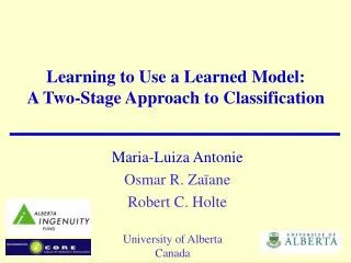
Learning to Use a Learned Model: A Two-Stage Approach to Classification. Maria-Luiza Antonie Osmar R. Zaïane Robert C. Holte. University of Alberta Canada. Outline. Prerequisites and Motivation Two stage approach to classification Rule-based features Class-based features

E N D
Learning to Use a Learned Model: A Two-Stage Approach to Classification Maria-Luiza Antonie Osmar R. Zaïane Robert C. Holte University of Alberta Canada
Outline • Prerequisites and Motivation • Two stage approach to classification • Rule-based features • Class-based features • Experimental results • Single label classification • Multi label classification • Conclusions ICDM 2006 Presentation
Association Rules A transaction is a set of items: T={ia, ib,…it} T I, where I is the set of all possible items {i1, i2,…in} D, the task relevant data, is a set of transactions. An association rule is: P Q, where P I, Q I, and PQ = PQ holds in D with support s and PQ has a confidence c in the transaction set D. Support(PQ) = Probability(PQ) Confidence(PQ)=Probability(Q/P) ICDM 2006 Presentation
■ ● ■ ● ■ ■ ● ● ■ ● ■ ● ■ ■ ● ● ■ ● ● ● ● Pruned Rules Applicable Rules Selected Rules Association Rules Associative Classifier Model input data into transactions Also modeled into transactions Unlabeled new objects Rule Pruning Rule Scoring Rule Generation Labeled objects Set of rules Set of transactions Set of rules <{i1, i2,…, ik},c> New object labelled New object Transactions (Training Data) ICDM 2006 Presentation
Motivation Rule-based model New object O{A,B,C} R1: D Class 1 – Confidence 95% R2: B E Class 2 – Confidence 90% R3: A D Class 1 – Confidence 90% R4: B C Class 3 – Confidence 90% R5: A Class 1 – Confidence 85% R6: A B Class 2 – Confidence 85% R7: B Class 2 – Confidence 80% R8: C Class 2 – Confidence 80% R9: A C Class 3 – Confidence 70% What strategy to use for a given application? R5: A Class 1 – Confidence 85% R6: A B Class 2 – Confidence 85% R7: B Class 2 – Confidence 80% R8: C Class 2 – Confidence 80% R4: B C Class 3 – Confidence 90% R9: A C Class 3 – Confidence 70% • First rule strategy (highest confidence): O is in Class 3 (R9:90%) • Average of confidences strategy: O is in Class 1 85%:{R5} • Number of applicable rules strategy: O is in Class 2 3:{R6, R7, R8} ICDM 2006 Presentation
Two-Stage Approach to Classification • First stage • Mine classification rules • Typical to associative classifier systems • Second stage • Use the set of rules to create new features (e.g.: average of confidences per class) • Learn a classification system in the new feature space • Classification of new objects ICDM 2006 Presentation
New object Training set ARM Set of Features Set of Rules Learner Training Learned Model Training set Set of Features … System Overview First Stage Classification Second Stage ICDM 2006 Presentation
■ ■ ■ ● ● {m1, m2,…, mj} <{m1, m2,…, mn},c> <{i1, i2,…, ik},c> {m1, m2,…, mj} n = #measures × #classes Object in item-space Applicable Rules Object in CF space Measures per class R5: A Class 1 – Confidence 85% O{A,B,C} R6: A B Class 2 – Confidence 85% R7: B Class 2 – Confidence 80% R8: C Class 2 – Confidence 80% ■ ● ■ ● ■ ■ ● ● R4: B C Class 3 – Confidence 90% R9: A C Class 3 – Confidence 70% Class 1 Class 2 Class 3 Avg conf. # rules Avg conf. # rules Avg conf. # rules Association Rules 85 1 81.6 3 80 2 Class-based Features (2SARC1) ICDM 2006 Presentation
{m1, m2,…, mj} ■ ● ■ ● ■ ■ ● ● <{m1, m2,…, mn},c> <{i1, i2,…, ik},c> n = #measures × #rules {m1, m2,…, mj} Object in item-space Association Rules Measures per rule Object in RF space R1: D Class 1 – Confidence 95% R2: B E Class 2 – Confidence 90% R3: A D Class 1 – Confidence 90% R4: B C Class 3 – Confidence 90% R5: A Class 1 – Confidence 85% R6: A B Class 2 – Confidence 85% R7: B Class 2 – Confidence 80% R8: C Class 2 – Confidence 80% R9: A C Class 3 – Confidence 70% Rule-based Features (2SARC2) ICDM 2006 Presentation
Experimental Results • Single label classification • Each object belongs to one class only • UCI datasets • Multi label classification • Each object belongs to one or more classes • Text classification – Reuters dataset • Our system • First stage – classification rule mining • Second stage – neural network learner ICDM 2006 Presentation
Experimental Results – Single Label UCI Datasets 20 sets Wins: 1 5 2 3 0 3 0 4 2 ICDM 2006 Presentation
Experimental Results – Single Label • We compared 9 classification systems on 20 datasets • Statistical analysis • In this type of experimental design careful consideration as to be given in choosing the appropriate statistical tools • The significance level has to be controlled to account for the multiple comparisons made • Friedman test, Wilcoxon signed ranked tests ICDM 2006 Presentation
Experimental Results – Single Label Count of wins, losses and ties for 2SARC1 when compared to the other systems 2SARC1 outperforms every other system on more than half of the UCI datasets ICDM 2006 Presentation
Experimental Results – Multi Label Reuters Dataset 10 classes Wins: 0 0 0 0 6 0 3 1 ICDM 2006 Presentation
Conclusions • We proposed a two-stage AC, where the scoring function is automatically learned • Advantages to the proposed method • It learns from the data how to classify • Versatile, general • Good performance (accuracy, BEP) • 2SARC1 performs better than 2SARC2 ICDM 2006 Presentation
Thank You! ICDM 2006 Presentation
Associative Classification • A set of association rules (R) • The rules are ordered by confidence and support • A new instance to be classified • Select from R a subset of rules R’ that match the new instance • Divide R’ in subsets based on the class label • R’C1, R’C2, …. R’Cn • Choose winning class(es) based on a scoring function ICDM 2006 Presentation
Classification • Predefined scoring functions • CBA [KDD’98] • Choose the first matching rule (highest confidence) • CMAR [ICDM’01] • For each R’C1, R’C2, …. R’Cn set • Computes a weighted chi-square • Chooses the class with the best score (best chi-square) • ARC-AC [MDMKDD’01] and ARC-BC [ICDM’02] • For each R’C1, R’C2, …. R’Cn set • Computes the average of the confidences • Chooses the class with the best score (best average confidence) ICDM 2006 Presentation
Experimental Results – Multi Label ICDM 2006 Presentation