Download
1 / 31
310 likes | 390 Views
Instructions for SAS v. 9.2. Save the programs to a common folder:. Make sure to retain (i.e. copy) the “FileFolder” which is required by other programs in order for them to work properly. In the instructions, the FileFolder is “I:Example”. Program Summary

E N D
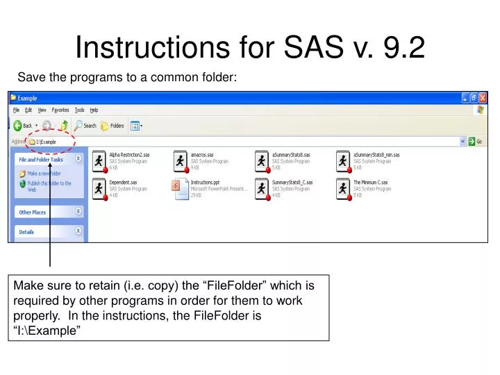
Instructions for SAS v. 9.2 Save the programs to a common folder: Make sure to retain (i.e. copy) the “FileFolder” which is required by other programs in order for them to work properly. In the instructions, the FileFolder is “I:\Example”
Program Summary Alpha Restriction.sas – Searches for critical values using the “alpha restricted method” over 1st and 2nd stage sample sizes with ranges specified by the user. amacros.sas – contains a set of macros utilized by other programs. aSummaryStats8.sas – is an algorithm that searches for a design that meets the user’s specifications, looking at average power similar to Chen and Ng (1998), over 8x8=64 accrual combinations. aSummaryStats8_min.sas – is an algorithm that searches for a design that meets the user’s specifications, requiring user specified minimum power over all accrual combinations. Dependent.sas – Characterizes the design under the case of associated (correlated) responses (i.e. Xr is not independent of Xs). The Minimum C.sas – Searches for critical values using the “Minimum C Method.” SummaryStats8_C.sas – is an algorithm that searches for a design that meets the user’s specifications, based on designs that use The Minimum C Method.
(1) Decide Which Method to Use: The Alpha Restriction or The Minimum C
An Example the Alpha Restriction Method Is Provided Below:
Open Alpha Restriction.sas using SAS software: You can enter the values of the parameters directly into the program. Since Greek letters are not accepted by the software, , etc. which are explicitly defined in the program introduction (not shown). The values of n1L, n1U, nL, and nU should encompass the anticipated sample sizes for stage 1 and 2. Don’t forget to provide the location of the “FileFolder” where the programs are located. Alternatively, the user can specify the parameters or change them after the program is run.
Running the program allows the user to explicitly see the values of the parameters being accepted by the computer (and their definitions). • Press the “Tab” key to move the cursor into and around the window. • Use the arrow keys to move within a specific field. Delete numbers and change values as usual. • When ready to begin computations, press the “Enter/Return” key in the last field (minimum sample size for stage 2).
SOME COMPUTATIONAL DETAILS: The computer will provide an initial printout of all of the combinations of stage 1 (n1) and cumulative stage 2 sample sizes (n). The total number of accrual combinations can be found on the last row of the Obs column. This will enable the user to approximately gauge the time for computations. In this example, there are 1681 combinations. Note that the lower bound for n is 50 when n1 is 40 since we desire at least 10 patients in Stage 2. The SAS log file can help the user see the progress of the computations by printing the size of the dataset OPERCHAR: NOTE: There were 175 observations read from the data set WORK.OPERCHAR. NOTE: There were 1 observations read from the data set WORK.OPERCHAR0. The computer should beep when finished. However, for large datasets, the log file can fill up causing computations to stop. If this happens, clear the window without saving. If this becomes annoying, the advanced user can use the “dm ‘log’ clear” option in the macro “cfind_CM2.”
When the computer finishes the computations (usually no longer than 5 or 10 minutes), it will printout some of the variables of interest in a dataset called “operchar” which stands for “operating characteristics.” The variable “CM” is defined as: CM=max(1 – Power Hr, 1 – Power Hs) which is used to help select critical values.
(2) Decide on a Searching Algorithm Having a large set of sample sizes and rejection boundaries, the user is now ready to narrow the search for a design that meets the desired specifications. There are currently two algorithms available for this purpose when Alpha Restriction.sas is used: (1) aSummaryStats8.sas, and (2) aSummaryStats8_min.sas. Both programs search through designs with accrual windows of size 8 at each stage (e.g. 21 – 28 Stage 1; 50 – 57 Stage 2). The total number of accrual combinations is 64 (8 possibilities for Stage 1 by 8 possibilities for Stage 2). aSummaryStats8.sas: First the algorithm finds a design with the smallest lower bound on n(1) that meets the users specification, using the average (mean over 8 possibilities) PET criteria. Then it searches for the smallest lower bound on n so that average power (over all 64 combinations) exceeds the user’s specifications when the alternative hypotheses are true. aSummaryStats8_min.sas: Is similar except it finds a design with the smallest lower bound on n(1) that meets the users specification, using the minimum value of PET over the 8 possibilities. Then it searches for the smallest lower bound on n so that minimum power (over all 64 combinations) exceeds the user’s specifications when the alternative hypotheses are true.
aSummaryStats8.sas Enter values of desired average PET and average power directly into the program. Alternatively, run the program and enter the parameters at that time.
Output from aSummaryStats8.sas The determined lower bound on the Stage 1 sample size is 17 since it is the smallest sample size that yields average PET ≥ 50%. The first stage accrual window is 17 to 24 (8 patients wide).
The lower bound in Stage 2 was determined to be 48 (accrual window from 48 to 55) since this is the smallest sample where average Power Hr ≥ 80% and average Power Hs ≥ 80%.
A Partial Listing of Critical Values and Individual Operating Characteristics
Statistical Summary of Design As a quality control measure, make sure the total number of accrual combinations is 64. If it is under 64, then the bounds provided by n1L, n1U, nL, or nU may be too restrictive. Also be alert to notices that state that the selected design is at one of these bounds. The maximum alpha ≤ 5% by design. However, a user may be uncomfortable with a design that has a particular accrual combination with power ≈ 75%.
Obtaining Characteristics for the Dependent Case Since calculating the operating characteristics for the dependent case is a bit time consuming, this data can be obtained by highlighting the code at the end of the program and running separately.
Statistical Summary of Design for Dependent Responses The average power decreases by less than 2%. However, the investigators may not be satisfied with power ≈ 73% in some circumstances.
aSummaryStats8_min.sas Program looks very similar.
The determined lower bound on the Stage 1 sample size is 23 since it is the smallest sample size that yields minimum PET ≥ 50%. The first stage accrual window is 23 to 30 (8 patients wide).
The lower bound in Stage 2 was determined to be 55 (accrual window from 55 to 62) since this is the smallest sample where: minimum Power Hr ≥ 80% and minimum Power Hs ≥ 80%.
A Partial Listing of Critical Values and Individual Operating Characteristics
Statistical Summary of Design The accepted design assures power at least 80% for all accrual combinations, but the sample size is increased accordingly.
Statistical Summary of Design for Dependent Responses These numbers drop slightly when the response variables are dependent. If the user is not satisfied, the required power can be increased to 82% to find a design and examined in the dependent case.
The Minimum C Method The program that uses the method of minimizing a C (for Cost function) is similar to Alpha Restriction.sas. The critical values in the second stage are found so that C = P(Type I error)2 + P(Type II under Hr)2 + P(Type II under Hs)2 is minimized for the various errors of concern (type I and II) Program is similar to the “Alpha Restricted Method” except the user does not specify a desired alpha. Currently, the user must enter values directly into the program. The dataset of prime interest is called “operchar” as before. Once this dataset is obtained, the investigator should use SummaryStats8_C.sas to obtain a satisfactory design.
SummaryStats8_C.sas This program requests a desired alpha at this stage.
The operating characteristics are not the same for this design as GOG 229E because the accrual window for this design is wider (8 patients) than it was for GOG 229E (5 patients).
Troubleshooting Assume we want a design that has PET>50% and power >90% If you want a demanding design but do not provide a broad enough range of sample sizes for the algorithms to find the desired design (i.e. n1L, n1U, nL, and nU are too narrow), then the algorithms will provide a “best” design from the cases examined, but it will not be adequate.
A warning should appear in cases where desired power is not attained. Obtained design is underpowered.
The design’s PET is only 39%. Power is close to the desired level. Use these results to help refine the search.