Download
1 / 17
170 likes | 309 Views
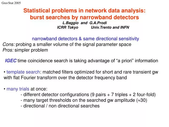
GravStat 2005. Statistical problems in network data analysis: burst searches by narrowband detectors L.Baggio and G.A.Prodi ICRR Tokyo Univ.Trento and INFN. narrowband detectors & same directional sensitivity Cons: probing a smaller volume of the signal parameter space

E N D
GravStat 2005 Statistical problems in network data analysis:burst searches by narrowband detectorsL.Baggio and G.A.Prodi ICRR Tokyo Univ.Trento and INFN narrowband detectors & same directional sensitivity Cons: probing a smaller volume of the signal parameter space Pros: simpler problem • IGEC time coincidence search is taking advantage of “a priori” information • template search: matched filters optimized for short and rare transient gw with flat Fourier transform over the detector frequency band • many trials at once: - different detector configurations (9 pairs + 7 triples + 2 four-fold) • - many target thresholds on the searched gw amplitude (30) • - directional / non directional searches
GravStat 2005 • … IGEC cont`d • data selection and time coincidence search: - control of false dismissal probability • - balance between efficiency of detection and background fluctuations • background noise estimation • - high statistics: 103 time lags for detector pairs • 104 – 105 detector triples • - goodness of fit tests with background model (Poisson) • blind analysis (“good will”): • - tuning of procedures on time shifted data by looking at all the observation time (no playground) • … what if evidence for a claim would appear ? • “GW candidates will be given special attention …” • - IGEC-2agreed on a blind data exchange (secret time lag)
GravStat 2005 Example: EX-NA background (one-tail 2 p-level 0.71) verified Poisson statistics For each couple of detectors and amplitude selection, the resampled statistics allows to test Poisson hypothesis for accidental coincidences. As for all two-fold combinations a fairly big number of tests are performed, the overall agreement of the histogram of p-levels with uniform distribution says the last word on the goodness-of-the-fit.
GravStat 2005 A few basics: confidence belts and coverage physical unknown experimental data
GravStat 2005 Feldman & Cousins (1998) and variations (Giunti 1999, Roe & Woodroofe 1999, ...) Im can be chosen arbitrarily within this “horizontal” constraint Fixed frequentistic coverage Freedom of choice of confidence belt
GravStat 2005 • Let • Poisson pdf: • Likelihood: • I fixed, solve for : • Compute the coverage Plot of the likelihood integral vs. minimum (conservative) coverage minN C(N ), with background counts Nb=0.01-10 Confidence intervals from likelihood integral
99% 95% Likelihood integral 85% N Example: Poisson background Nb = 7.0
GravStat 2005 • Let • Poisson pdf: • Likelihood: • I fixed, solve for : • Compute the coverage Plot of the likelihood integral vs. minimum (conservative) coverage minN C(N ), with background counts Nb=0.01-10 Confidence intervals from likelihood integral
GravStat 2005 Multiple configurations/selection/grouping within IGEC analysis
GravStat 2005 expected found Resampling statistics of accidental claims event time series coverage “claims” 0.90 0.866 (0.555) [1] 0.95 0.404 (0.326) [1] Easy to set up a blind search
GravStat 2005 Keep track of the number of trials (and their correlation) ! IGEC-1 final results consist of a few sets of tens of Confidence Intervals with min{C}=95% • the “false positives” would hide true discoveries requiring more than 5 two-sided C.I. to reach 0.1% confidence for rejecting H0 the procedure was good for Upper Limits, but NOT optimized for discoveries • Need to decrease the “false alarm probability” (type I error)
Freedom of choice of confidence belt Fine tune of the false alarm probability
GravStat 2005 Example: confidence belt from likelihood integralPoisson background Nb = 7.0Min{C}=95% P{false alarm}< 5 % P{false alarm} < 0.1% 1 - C(N )
GravStat 2005 What false alarm threshold should be used to claim evidence for rejecting the null H0? • control the overall false detection probability: • Familywise Error Rate < requires single C.I. with P{false alarm} < /m • Pro: rare mistakes • Con: high detection inefficiency • control the mean False Discovery Rate: • R = total number of reported discoveries • F+=actual number of false positives • Benjamini & Hochberg (JRSS-B (1995) 57:289-300) • Miller et. al. (A J 122: 3492-3505 Dec 2001;http://arxiv.org/abs/astro-ph/0107034)
FDR control The p-values are uniformly distributed in [0,1] if the assumed hypothesis is true Usually, the alternative hypothesis is not known. However, the presence of a signal would contribute to bias the p-values distribution. pdf Typically, the measured values of p are biased toward 0. 1 signal background p-level
Sketch of Benjamini & Hochberg FDR control procedure • compute p-values {p1, p2, …pm} for a set of tests, and sort them in creasing order; • choose your desired bound q on <FDR>; • determine the threshold T= pk by finding the index k such that pj<(q/m) j • for every j>k; • OK if p-values are independent or positively correlated • in case NO signal is present (H0 is true), the procedure is equivalent to the control of the FamilyWise Error Rate at confidence < q m counts reject H0 q p-value T
GravStat 2005 Open questions • check the fluctuations of the random variable FDR with respect to the mean. • check how the expected uniform distribution of p-values for the null H0 can be biased (systematics, …) • would the colleagues agree that overcoming the threshold chosen to control FDR means & requires reporting a rejection of the null hypothesis ? To me rejection of the null is a claim for an excess correlation in the observatory at the true time, not taken into account in the measured noise background at different time lags. It could NOT be gws, but a paper reporting the H0 rejection is worthwhile and due.