Download
1 / 17
170 likes | 255 Views
RECENT STUDIES OF OXYGEN-IODINE LASER KINETICS. Azyazov V.N. and Pichugin S.Yu. P.N. Lebedev Physical Institute,Samara Branch, Russia. Heaven M.C. Emory University, Atlanta, USA. O 3 -SF 6 -N 2 O. О 2 ( а 1 ) -O( 1 D)-I 2 ( или CH 3 I).

E N D
RECENT STUDIES OF OXYGEN-IODINE LASER KINETICS Azyazov V.N. and Pichugin S.Yu. P.N. Lebedev Physical Institute,Samara Branch, Russia Heaven M.C. Emory University, Atlanta, USA
O3-SF6-N2O О2(а1 )-O(1D)-I2(или CH3I) Chemical OIL (COIL)Cl2+НО2-HCl + Cl-+О2(1 )PО2 100 Тор, =[О2(1)]/[O2]50 % Nozzle + DischargeOIL (DOIL)О2(Х) + е О2(1 )+ еPО2 10 Тор, 20 % О2 О2 О2(1 ), О - Resonator NO2 I2 UV photolysis PhotolyticOIL (PhOIL)О3 + hv О2(1 )+ O(1D)PО2 1 Тор, 90 %
The low-pressure flow cell apparatus with a jet-type SOG Dependence of the I* concentration on the distance along the flow for w=3 %, O2:N2=1:1
Testing role of O2(1) by addition of CO2 Quenching of O2(1) has a minimal effecton the I2 dissociation rate O2(1) I* Reducing [O2(1)] by an order of magnitude caused a slight increasing of the dissociation time
Role of I2(B) in the iodine dissociation COIL active medium luminescence spectra in the visible range recorded with a resolution of 1 nm at Pc = 2.3 Torr, I2 =0.5%, N2:O2=1:1 Branching fraction GB=5105 s-1 , Gb=0.08 s-1 I2(A, A') + O2(a) I2(1Π1u) + O2(X) I + I + O2(X), approx=100 % I2(B) + M I + I + M, < 1 %
Estimation of excitation probabilitiesfrom Barnault et al. measurements I*+ I2 I+I2(X,v) v -excitation probability of v-th vibrational level m≤v≤n= v25»0.1 10<v23»0.9 (0 for dashed curve) Standard dissociation model with v25»0.1 can not provide observed dissociation rates in COIL medium. About 20 molecules of O2(a) consumed to dissociate one I2 molecule if standard model is predominant dissociation pathway.
Pump-probe technique used to study OIL kinetics Nd/YAG Pumped Dye Laser Quenching gas I2+Ar Delay Generator Monochromator Digital Oscilloscope Ge Pump Fluorescence cell Excimer laser Light baffles Rate ofI2(A') quenching (Rq) depends on CO2 partial pressureРСО2atPAr=50 Torr, РI2=0.013 TorrandT=300 K KCO2= 8.510-13cm3/s KAr= 2.710-14cm3/s KO2= 6 10-12cm3/s KI2= 4.810-11cm3/s
Branching fraction for O2(1) from O(1D)+N2O & O(3P)+N2O N2O,NO2 or O3 Power meter 1268 nm filter 193 or 248 nm Ge photo- detector Pump O2(1) formation: N2O +193 nm O(1D) + N2 O(1D) + N2O N2 + O2(1) ? O(3P) + NO2 NO + O2(1) ? O3 +248 nm O(1D) + O2(1) O2(1) O2(3)+1268 nm Yield O(1D) + N2O N2 + O2(1) 100 % O(3P) + NO2 NO + O2(1) <10 % Typical temporal profiles of the 1268 nm emission intensities for the N2O photolysis experiment (IN2O) –PN2O=207 Torr, PAr=407 Torr and for the O3 photolysis experiment (IO3)-PN2=755 Torr, PAr=1.3 Torr
Quenching I(2P1/2)by О(3Р), О3 N2O + 193 нм N2 + O(1D) O(1D) + N2O N2 + O2(1) NO + NO O3 +248 nm O(1D) + O2(1) O(1D) + CO2(N2) O(3P) + CO2(N2) I2(X) + O(3P) IO+ I(2P3/2) IO + O(3P) O2(3)+I(2P3/2) I(2P3/2) + O2(1) I(2P1/2) + O2(3) I(2P1/2) +O(3P) I(2P3/2) +О(3P) I(2P1/2) +O3 products I(2P1/2 ) I(2P3/2 )+ h (= 1315 nm) Dashed lines are calculations at KO=1.210-11 cm3/s KO3=1.810-12 cm3/s
Quenching I(2P1/2) by NO2, N2O4&N2OCF3I + h (248 nm) CF3 + I(2P1/2) sNO2=2.85x10⁻¹⁹ cm2NO2 + h (248 nm) O + NO sNO2=2x10-20 cm2N2O4 + h (248 nm) NO2+ NO2sN2O4= 80sNO2 O+ NO+NO2 KN2O4= (3.70.5)×10-13cm3/s KNO2= (2.90.3)×10-15cm3/s KN2O= (1.30.1)×10-15cm3/s
Quenching ofO2(a1)in the presence О2andO(3P) O(3P) + O2(1) + O2 O(3P) + 2O2 O3 +h(248 nm)O(1D)+O2(1) O(3P) + O2(X) O2(1) O2(3)+ h (1268 nm) Temporal emission intensity ofO2(1) at PO3=2.4 Torr, Ptot=773 Torr. Dashed lines are calculations at K=1.1x10⁻³¹ cm6/s. NO2 emission intensity near to 600 nm at PO3=2.4 Torr, PN2O=2.8 Torr, Ptot=762 Torr
Conclusions The total excitation probabilities of I2(X,v) in reaction I* + I2I + I2(X,v>10) arev25 0.1 and 10<v<25 0.9 Standard dissociation model with v250.1 can not provide observed dissociation rates in COIL medium. About 20 molecules of O2(a) consumed to dissociate one I2 molecule if standard model is predominant dissociation pathway. I2(B) and takes a minor part in iodine dissociation and O2(b) does not play a noticeable role in I2(B) formation I2 dissociation pathway involvingO2(b)state is not major channel
Conclusions • Measured kinetic constants: I2(A) + CO2 I2(X) + CO2 (8.50.9)10-13cm3/s I2(A) + O2 I2(X) + O2 (6.00.6)10-12cm3/s I2(A) + I2 I2(X) + I2(4.80.9)10-11cm3/s I2(A) + Ar I2(X) + Ar (2.70.3)10-14cm3/s О2(b)+ CO2 О2(а)+ CO2 (6.10.5)10-13cm3/s О2(b)+ O3 products(1.90.2)10-11cm3/s I(2P1/2) + O(3P) I + O(3P) (1.2±0.1)10-11cm3/s I(2P1/2) + O3 products (1.8±0.4)10-12cm3/s I(2P1/2) + NO2 I + NO2(2.9±0.3)10-15cm3/s I(2P1/2) + N2O4 I + N2O4(3.7±0.5)10-13cm3/s I(2P1/2) + N2O I + N2 O (1.3±0.1)10-15cm3/s O2(a1) + O(3P) + O2 O(3P) + 2O2 (1.1±0.2)10-31cm6/s • Yield ofO2(a1) in reactions O(1D) + N2O N2 + O2(3) or O2(1)- 1±0.12 O(3Por1D) + NO2 NО + O2(3) or O2(1)-< 0.1
DevelopedI2 dissociation model O2(a,v=1)+I2(X)O2(X)+I2(A’) (95) O2(a,v=2)+I2(X)O2(X)+I2(A) (96) O2(a)+I2(A’,A) O2(X)+2I (25) I* + I2 I + I2(10<v<25) (33) I2(10<v<25)+O2(a)O2(X)+I2(A’,A) (101) O2(a,v=3)+I2(X)O2(X)+2I (97) O2(a,v=1)+I2(X,v15)O2(X)+2I (102) O2(a,v=2)+I2(X,v8) O2(X)+2I (103) O2(b) + I2(X) O2(X) + 2I (21) Heidner et al. model O2(a)+I2(X)O2(X)+ I2(20<v<45) (32) I2(20<v<45)+O2(a)O2(X)+2I (34) I* + I2 I + I2(25<v<45) (33) Potential energy curves of I2. The red and blue arrows show the excitation pathways of energy states lying bellow and above the I2 dissociation limit, respectively. The inscriptions above arrows denote the reaction producing excitation
Conclusions A model that involves excitation of I2(A’,A) by reactions O2(a,v=1)+I2(X)O2(X)+I2(A’) (95) O2(a,v=2)+I2(X)O2(X)+I2(A) (96) O2(a)+I2(A’,A) O2(X)+2I (25) I* + I2 I + I2(10<v<25) (33) I2(10<v<25)+O2(a)O2(X)+I2(A’,A) (101) yields results that are in reasonable agreement with the flow tube experiments.