B-2 Multifragmentation – 0 Introduction

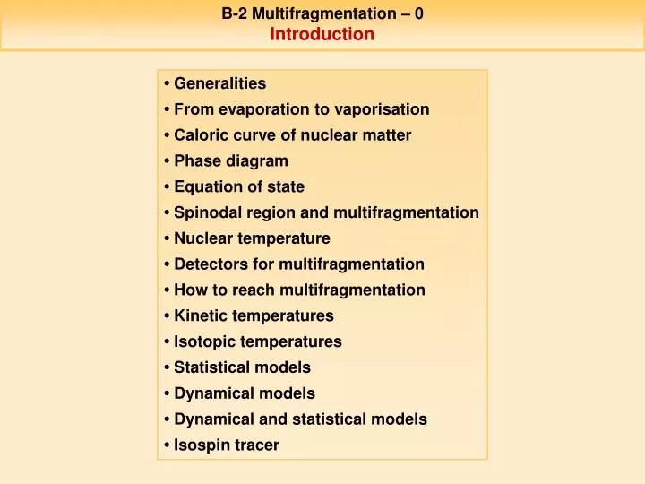
1. B-2 Multifragmentation – 0 Introduction • Generalities • From evaporation to vaporisation • Caloric curve of nuclear matter • Phase diagram • Equation of state • Spinodal region and multifragmentation • Nuclear temperature • Detectors for multifragmentation • How to reach multifragmentation • Kinetic temperatures • Isotopic temperatures • Statistical models • Dynamical models • Dynamical and statistical models • Isospin tracer

2. B-2 Multifragmentation – 1 Generalities preequilibrium emission Definition: decay of a composite nuclear system into several heavy fragments (3  Z  30). It is a very fast decay mode, the time scales involved are at most of the order of several hundred fm/c (1 fm/c = 3.10-24 s). J. Bondorf et al., Phys. Rep. 257(1995)133 At freeze-out: density r ~ r0/3 temperature T ~ 5 MeV excitation energy E* ~ 4-6 AMeV

3. B-2 Multifragmentation – 2 From evaporation to vaporisation INDRA Au+Au at 60 AMeV quasi-projectile multifragmentation DE evaporation towards vaporisation peripheral central E ALADIN multiplicity of IMF’s multifragmentation vaporisation evaporation AMeV Zbound = Z with Z 2 A.Schüttauf et al., Nucl. Phys. A 607 (1996) 457 central peripheral

4. B-2 Multifragmentation – 3 Caloric curve of nuclear matter Caloric curve of nucleus Caloric curve of water gas Temperature (MeV) liquid Excitation energy per Nucleon (MeV) J. Pochodzalla et al., Phys. Rev. Lett. 75(1995)1040

5. B-2 Multifragmentation – 4 Phase diagram 1.The liquid phase: nuclear matter in its ground state, at low temperatures and densities. 2.The condensed phase: supposed to be cold matter at high densities where nucleons are organized into a crystal. 3. The gaseous phase:appears at fairly high temperatures and low densities at which the nuclei evaporate into a hadron gas. 4. The plasma phase:deconfined mixture of quarks and gluons coming from the dissociation of hadrons into their elementary constituents ( ~ 5-10 0 , T~150 MeV)

6. B-2 Multifragmentation – 5 Equation of state Generally, the equation of state of a system is a relation between three thermodynamicalvariables. For the nuclear matter: density temperature binding energy of the infinite nuclear matter in its ground state internal energy compression energy at T=0 thermal energy Saturation point: For a sufficiently heavy nucleus, increasing its number of constituents does not modify the density of nucleons in its central part. The saturation density 0 is independent of the nuclear size. 0 = 0.17  0.02 nucleon.fm-3 ( R=r0.A1/3 with r0=1.2fm )

7. B-2 Multifragmentation – 6 Equation of state Compression energy Compressibility Low K(~ 200 MeV)  softequation of state (one has to give relatively little compression energy to reach high densities) High K(~ 400 MeV)  hardequation of state Recent experimental results in heavy-ion collision studies seem to favor a soft equation of state. A. Andronic et al., Nucl. Phys. A 661(1999)333c, C. Fuchs et al., Phys. Rev. Lett. 86(2001)1974 Any equation of state is based on the knowledge of the elementary interactions between the constituents.  The nucleon-nucleon interaction potential has a dominant term that is repulsive at short range (  0.5 fm ) and attractive at longer range (  0.8 fm )  NN potential ~ molecule potential  EoS (infinite nucleon system) ~ EoS (Van der Waals gas)  isotherms, liquid-gas phase transition Problem: the fermionic nature of the nucleons  simple real fluid  approximate theoretical description from the saturation point as the balance between the attractive part of the nuclear interaction potential and the repulsion between nucleons.

8. B-2 Multifragmentation – 7 Spinodal region and multifragmentation isotherms spinodal region Nuclei reaching the spinodal region blow up into several fragments, undergoing a reaction process of multifragmentation. This decay mode is a way to study the transition between the liquid and gas phases. Coexistence zone of liquid-gas phases for T<Tc = 17.9 MeV with a spinodal region characterized by a mechanically instable regime with a negative compressibility K = -1/V.dP/dV

9. B-2 Multifragmentation – 8 Nuclear temperature Definition of the temperature provided by statistical mechanics: This definition is applicable to any isolated system, like a nuclear system if one regards the very short range of the nuclear forces. Requirement: full statistical equilibrium  Difficult to achieve due to the short time range of the reaction, the finite size of the system, the complex dynamics, and the various collisions that occur in a collision.  Experimental results interpreted as a signal of an equilibrium A. Schüttauf et al., Nucl. Phys. A 607(1996)457 binding energies Isotopic temperatures Experimental thermometers Maxwell-Boltzmann distribution: yield constant containing the spins and A’s yields of the species Kinetic temperatures E

10. B-2 Multifragmentation – 9 Detectors for multifragmentation 4p detectors Spectrometers ALADIN INDRA EOS MINIBALL

11. B-2 Multifragmentation – 10 How to reach multifragmentation maximum fragment production in central collisions A.Schüttauf et al., Nucl. Phys. A 607 (1996) 457

12. B-2 Multifragmentation – 11 Kinetic temperatures Au+Au at 600 AMeV, mid-peripheral collisions Maxwell-Boltzmann fit: T. Odeh, PhD thesis, University Frankfurt (1999)

13. B-2 Multifragmentation – 12 Isotopic temperatures + Au+X at 600 AMeV T. Odeh, PhD thesis, University Frankfurt (1999)

14. B-2 Multifragmentation – 13 Statistical models • Assumption of an equilibrated source emitting fragments in either microcanonical, canonical or grand canonical ensembles. • The break-up process is either spontaneous, all fragments are emitted at the same time, or, it is a slow process, the fragments are emitted sequentially. Example: the SMM code (Statistical Multifragmentation) J. Bondorf et al., Phys. Rep. 257(1995)133 It is a mixed approach, based on the microcanonical assumption (conservation of the total energy) and using canonical prescriptions of partitions. It assumes that fragments are distributes in a certain available volume V (supposed to be the freeze-out volume) following Boltzmann statistics. The density of the freeze-out corresponds to the coexistence region of the phase diagram. The internal structure of the fragments is described by means of the liquid drop model. The mass and charge are exactly conserved with every single event. The produced fragments may be excited and may also undergo a secondary decay. It depends on their mass: fragments up to oxygen can de-excite by breaking into several single nucleons and light clusters. Heavier, excited fragments can evaporate light particles.

15. B-2 Multifragmentation – 14 Statistical models Experimental results and statistical model Multiplicities Temperature THeLi Good agreement for the fragments but not for the light particles! T. Odeh, PhD thesis, University Frankfurt (1999)

16. B-2 Multifragmentation – 15 Dynamical models The dynamical models follow the time evolution of the system, from the collision until the freeze-out. Example: the INC code (Intra-Nuclear Cascade) J. Cugnon, Phys. Rev. C 22 (1980) 1885 D. Doré et al., Phys. Rev. C 63 (2001) 034612 Nucleus-nucleus version! The code does not follow the state of the ensemble of cascade particles but the state of each cascade particles as a function of time. This permits to take into account in a total explicit way the motion of the nucleons and the collisions it generates. At the beginning, the nucleons are randomly positioned in a sphere. Particles move along straight line trajectories until two of them reach their minimum distance of approach dmin. All the particles are followed in this way until a stopping time tstop. This time is determined from the excitation energy of the remnant, the emission anisotropy , and the saturation of the cumulative numbers of collisions or escaping particles. In the nucleus-nucleus case, the stopping time has been set to 40 fm/c.

17. B-2 Multifragmentation – 16 Dynamical and statistical models Combination of dynamical and statistical models yield cascade + multifragmentation cascade E multifragmentation

18. B-2 Multifragmentation – 17 Isospin tracer • Ru+Zr and Zr+Ru at 400 AMeV • 40Zr and 44Ru have stable isotopes with the same mass A = 96. Zr+Ru or Ru+Zr relative abundance of protons RZ (Zr+Zr) = +1 and RZ (Ru+Ru) = -1 RZ = 0  full mixing

19. B-2 Multifragmentation – 18 Isospin tracer Relative abundance of protons as a function of… … rapidity for central collisions … centrality of the collisions F. Rami et al., Phys. Rev. Lett. 84(2000)1120