Download
1 / 13
130 likes | 138 Views
The General Linear Model. Or, What the Hell’s Going on During Estimation?. What we hope to cover: Extension of linear to multiple regression Matrix formulation of multiple regression; residuals and parameter estimates General and Generalised Linear Models

E N D
The General Linear Model Or, What the Hell’s Going on During Estimation?
What we hope to cover: • Extension of linear to multiple regression • Matrix formulation of multiple regression; residuals and parameter estimates • General and Generalised Linear Models • Overdetermined models and the pseudoinverse solution • Specific application to fMRI and basis sets
Multiple Regression Last time, David talked about linear regression – that is determination of a linear relationship between a single dependent and a single independent variable, of the form: Y = βX + c For example, we might think that the number of papers a researcher publishes a year (Y) is related to how hard working he/she is (X) and we can attempt to determine the regression coefficient (β) which reflects how much of an effect X has on Y. This approach can be extended to account for multiple variables, such as how friendly you were to potential reviewers at a recent conference, and combined in a linear fashion: Y = β1x1 + β2x2 …… βLxL + ε(1)
Multiple Regression The β parameters reflect the independent contribution of each explanatory variable to Y, that is the amount of variance accounted for by that variable after all the other variables have been accounted for. For example – one might see a negative correlation between height and hair length. However, if we add an explanatory variable reflecting gender (a categorical or dummy variable) then we see that the apparent correlation above actually reflects that, on average, men are taller than women, whilst women tend to have longer hair, and that height has no independent predictive value for hair length. The regression surface (the equivalent of the slope line in simple regression) expresses the best prediction of the dependent variable, Y, given the explanatory variables (Xs). However, observed data will deviate from this regression surface, the deviation from the corresponding point being termed the residual.
Matrix Formulation of Multiple Regression Y1x11 … x1 l… x1 L11 :: … : … : : : Yj = xj 1 … xj l… xj Ll + j ::… :… : : : YJxJ 1… xJ l … xJ LLJ Y = X×b + e Writing out equation (1) for each observation of Y gives a series of simultaneous equations: Y1 = x1 1 β1 + . . . + x1 lβl + . . . + x1 L + ε1 : = : Yj = xj1β1 + . . . + xj lβl + . . . + xj L + εj : = : YJ = xJ1β1 + . . . + xJlβl + . . . + xJL + εJ In Matrix Form: Design Matrix Observed data Parameters Residuals
Parameter Estimation Typically the simultaneous equations shown before cannot be fully solved (i.e. with ε= 0), so we aim to achieve the best between model and data, by minimising the sum of squares of the residuals – this is the least squares estimate: Residual sum of squares Minimised when which is the lth row of so the least squares estimates satisfy the normal equations giving (2)
Extension to General and Generalised Linear Models • Multiple Regression (as with many parametric tests, including t- and F-tests, ANOVAs, ANCOVAs etc.) is basically a limited form of a generalised linear model (GLM), with certain constraints, particularly:- • Only 1 dependent variable can be analysed • It assumes that errors are independently, identically and normally distributed, with mean 0 and variance σ2 (shown as ~ iid Ν(0,σ2))
Extension to General and Generalised Linear Models The General Linear Model allows linear combinations of multiple dependent variables (multivariate statistics), replacing the Y vector of J observations of a single Y variable with a matrix of J observations of N different variables – similarly the β vector is replaced with a JxN matrix. However, whilst a fMRI experiment could be modelled with a Y matrix reflecting BOLD signal at N voxels over J scans, SPM takes a mass univariate approach – that is each voxel is represented by a column vector of observations over scans and processed through the same model. Generalised Linear Models (GLMs) do not assume spherical error distributions, and hence can be utilised in order to correct for temporal correlations (this will be covered in a later talk).
Overdetermined Models and Pseudoinversion If the design matrix (X) has columns which are not linearly independent then it is rank deficient and XTX has no inverse. In this case there are an infinite number of parameter estimates which can describe this model, with an infinite number of least square estimates which satisfy (2) – such a model is said to be overdetermined. Since we hope for a single set of parameters in order to construct our significance tests a constraint must be applied to the estimates – the key point being then that inference can only be meaningfully engaged in when considering functions of those parameters not influenced by the chosen constraint. SPM uses a pseudoinverse solution, and the pseudoinverse (XTX)- can be substituted for (XTX)-1 in eq. (2)
GLM and fMRI Models We have looked so far at multiple regression and the general linear model in a fairly abstract context. We shall now think about how it applies to fMRI experiments: Y = X . β + ε Design matrix – formed of several components which explain the observed data: Timing information consisting of onset vectors Omj and duration vectors Dm Impulse response function hm describing the shape of expected BOLD response Other regressors e.g. movement parameters Parameters defining the contribution of each component of the design matrix to the model. These are estimated so as to minimise the error, and are used to generate the contrasts between conditions (next week). Error - the difference between the observed data and the model defined by Xβ. In fMRI these are not assumed to be spherical (temporal correlations). Observed data – SPM uses a mass univariate approach – that is each voxel is treated as a separate column vector of data.
GLM and fMRI Models The design of the experiment is principally defined by : The stimulus function Sm, representing occurrence of a stimulus type in each of a series of contiguous time bins for each trial type m. This is generated by SPM 2 from the onset vector Omj and the duration vector, Dm. The impulse response function, hmfor trial type m. The observed data, Y, is then expressed as: Y = ( Σ hm conv Sm) + ε The impulse response functions are not known, but SPM assumes that they can be modelled as linear combinations of basis functions bi such that: hmi = bi . βmi A typical basis function set might comprise the haemodynamic response function (HRF) and its partial derivatives with respect to time and dispersion.
GLM and fMRI Models How does this look with data? Observed data Model (green and red) and true signal (blue) Error + noise – set parameters to minimise this
Summary • The general linear model is a powerful statistical tool allowing determination of multiple parameters predicting multiple dependent variables. Many other parametric tests are special cases of the general linear model (t-tests, ANOVAs, F-test, regression) • The design matrix contains the information about the designed aspects of the experiment which may explain the observed data. • Minimising the sum of square differences between the modelled and observed data allows determination of the optimal parameters for the model. • The parameters can then be utilised to construct F- and t-tests to determine the significance of contrasts between experimental factors (more next week). • In fMRI we convolve the information about impulse response functions and the timing of different trial types to give the design matrix. We must also utilise a Generalised Linear Model to allow correction for temporal correlations over scans (more in a few weeks).