Download
1 / 50
500 likes | 624 Views
Scale-up of Cortical Representations in Fluctuation Driven Settings. David W. McLaughlin Courant Institute & Center for Neural Science New York University http://www.cims.nyu.edu/faculty/dmac/ IAS – May‘03. I. Background. Our group has been modeling a local patch (1mm 2 ) of a

E N D
Scale-up of Cortical Representationsin Fluctuation Driven Settings David W. McLaughlin Courant Institute & Center for Neural Science New York University http://www.cims.nyu.edu/faculty/dmac/ IAS – May‘03
I. Background Our group has been modeling a local patch (1mm2) of a single layer of Primary Visual Cortex Now, we want to “scale-up” David Cai David Lorentz Robert Shapley Michael Shelley Louis Tao Jacob Wielaard
Local Patch 1mm2
Lateral Connections and Orientation -- Tree Shrew Bosking, Zhang, Schofield & Fitzpatrick J. Neuroscience, 1997
From one “input layer” to several layers Why scale-up?
II. Our Large-Scale Model • A detailed, fine scale model of a local patch of input layer of Primary Visual Cortex; • Realistically constrained by experimental data; • Integrate & Fire, point neuron model (16,000 neurons per sq mm). Refs: --- PNAS (July, 2000) --- J Neural Science (July, 2001) --- J Comp Neural Sci (2002) --- J Comp Neural Sci (2002) --- http://www.cims.nyu.edu/faculty/dmac/
III. Cortical Networks Have Very Noisy Dynamics Strong temporal fluctuations On synaptic timescale Fluctuation driven spiking
Fluctuation-driven spiking (fluctuations on the synaptic time scale) Solid: average ( over 72 cycles) Dashed: 10 temporal trajectories
IV. Coarse-Grained Asymptotic Representations For “scale-up” in fluctuation driven systems
A Regular Cortical Map ---- 500 ----
For the rest of the talk, consider one coarse-grained cell, containing several hundred neurons
We’ll replace the 200 neurons in this CG cell by an effective pdf representation • For convenience of presentation, I’ll sketch the derivation of the reduction for 200 excitatory Integrate & Fire neurons • Later, I’ll show results with inhibition included – as well as “simple” & “complex” cells.
N excitatory neurons (within one CG cell) • all toall coupling; • AMPA synapses (with time scale ) t vi = -(v – VR) – gi (v-VE) t gi = - gi + l f (t – tl) + (Sa/N) l,k (t – tlk) (g,v,t) N-1 i=1,N E{[v – vi(t)] [g – gi(t)]}, Expectation “E” taken over modulated incoming (from LGN neurons) Poisson spike train.
t vi = -(v – VR) – gi (v-VE) t gi = - gi + l f (t – tl) + (Sa/N) l,k (t – tlk) Evolution of pdf -- (g,v,t): t = -1v {[(v – VR) + g (v-VE)] } + g {(g/) } + 0(t) [(v, g-f/, t) - (v,g,t)] + N m(t) [(v, g-Sa/N, t) - (v,g,t)],where 0(t) = modulated rate of incoming Poisson spike train; m(t) = average firing rate of the neurons in the CG cell = J(v)(v,g; )|(v= 1) dg where J(v)(v,g; ) = -{[(v – VR) + g (v-VE)] }
t = -1v {[(v – VR) + g (v-VE)] } + g {(g/) } + 0(t) [(v, g-f/, t) - (v,g,t)] + N m(t) [(v, g-Sa/N, t) - (v,g,t)], N>>1; f << 1; 0 f = O(1); t = -1v {[(v – VR) + g (v-VE)] } + g {[g – G(t)]/) } + g2/ gg + … where g2 = 0(t) f2 /(2) + m(t) (Sa)2 /(2N) G(t) = 0(t) f + m(t) Sa
Moments • (g,v,t) • (g)(g,t) = (g,v,t) dv • (v)(v,t) = (g,v,t) dg • 1(v)(v,t) = g (g,tv) dg where (g,v,t) = (g,tv) (v)(v,t) Integrating (g,v,t) eq over v yields: t (g) =g {[g – G(t)]) (g)} + g2 gg (g)
Fluctuations in g are Gaussian t (g) =g {[g – G(t)]) (g)} + g2 gg (g)
Integrating (g,v,t) eq over g yields: t (v) = -1v [(v – VR) (v) + 1(v)(v-VE) (v)] Integrating [g (g,v,t)] eq over g yields an equation for 1(v)(v,t) = g (g,tv) dg, where (g,v,t) = (g,tv) (v)(v,t)
t 1(v) = - -1[1(v) – G(t)] + -1{[(v – VR) + 1(v)(v-VE)] v 1(v)} + 2(v)/ ((v)) v [(v-VE) (v)] + -1(v-VE) v2(v) where 2(v) = 2(v) – (1(v))2 . Closure: (i) v2(v) = 0; (ii) 2(v) = g2
Thus, eqs for (v)(v,t) & 1(v)(v,t): t (v) = -1v [(v – VR) (v)+ 1(v)(v-VE) (v)] t 1(v) = - -1[1(v) – G(t)] + -1{[(v – VR) + 1(v)(v-VE)] v 1(v)} + g2 / ((v)) v [(v-VE) (v)] Together with a diffusion eq for (g)(g,t): t (g) =g {[g – G(t)]) (g)} + g2 gg (g)
But we can go further for AMPA ( 0): t 1(v) = - [1(v) – G(t)] + -1{[(v – VR) + 1(v)(v-VE)] v 1(v)} + g2/ ((v)) v [(v-VE) (v)] Recall g2 = f2/(2) 0(t) + m(t) (Sa)2 /(2N); Thus, as 0, g2 = O(1). Let 0: Algebraically solve for 1(v) : 1(v) = G(t) + g2/ ((v)) v [(v-VE) (v)]
Result: A Fokker-Planck eq for (v)(v,t): t (v) = v{[(1 + G(t) + g2/ ) v – (VR + VE (G(t) + g2/ ))](v) + g2/ (v- VE)2v(v)} g2/ -- Fluctuations in g Seek steady state solutions – ODE in v, which will be good for scale-up.
Remarks: (i) Boundary Conditions; (ii) Inhibition, spatial coupling of CG cells, simple & complex cells have been added; (iii) N yields “mean field” representation. Next, use one CG cell to (i) Check accuracy of this pdf representation; (ii) Get insight about mechanisms in fluctuation driven systems.
Bistability and Hysteresis • Network of Simple and Complex — Excitatory only N=16! N=16 MeanDriven: FluctuationDriven: Relatively Strong Cortical Coupling:
Bistability and Hysteresis • Network of Simple and Complex — Excitatory only N=16! MeanDriven: Relatively Strong Cortical Coupling:
Three Levels of Cortical Amplification : • 1) Weak Cortical Amplification • No Bistability/Hysteresis • 2) Near Critical Cortical Amplification • 3) Strong Cortical Amplification • Bistability/Hysteresis • (2) (1) • (3) • I&F • Excitatory Cells Shown • Possible Mechanism • for Orientation Tuning of Complex Cells • Regime 2 for far-field/well-tuned Complex Cells • Regime 1 for near-pinwheel/less-tuned With inhib, simple & cmplx (2) (1)
New Pdf for fluctuation driven systems -- accurate and efficient • (g,v,t) -- (i) Evolution eq, with jumps from incoming spikes; (ii) Jumps smoothed to diffusion in g by a “large N expansion” • (g)(g,t) = (g,v,t) dv -- diffuses as a Gaussian • (v)(v,t) = (g,v,t) dg ; 1(v)(v,t) = g (g,tv) dg • Coupled (moment) eqs for (v)(v,t) & 1(v)(v,t) , which are not closed [but depend upon 2(v)(v,t) ] • Closure -- (i) v2(v) = 0; (ii) 2(v) = g2 , where 2(v) = 2(v) – (1(v))2 . • 0 eq for 1(v)(v,t) solved algebraically in terms of (v)(v,t), resulting in a Fokker-Planck eq for (v)(v,t)
Scale-up & Dynamical Issuesfor Cortical Modeling of V1 • Temporal emergence of visual perception • Role of spatial & temporal feedback -- within and between cortical layers and regions • Synchrony & asynchrony • Presence (or absence) and role of oscillations • Spike-timing vs firing rate codes • Very noisy, fluctuation driven system • Emergence of an activity dependent, separation of time scales • But often no (or little) temporal scale separation
Fluctuation-driven spiking (very noisy dynamics, on the synaptic time scale) Solid: average ( over 72 cycles) Dashed: 10 temporal trajectories
Simple Complex Expt. Results Shapley’s Lab (unpublished) 4B # of cells 4C CV (Orientation Selectivity)
Incorporation of Inhibitory Cells • 4 Population Dynamics • Simple: • Excitatory • Inhibitory • Complex: • Excitatory • Inhibitory • Complex Excitatory Cells • Mean-Driven
Incorporation of Inhibitory Cells • 4 Population Dynamics • Simple: • Excitatory • Inhibitory • Complex: • Excitatory • Inhibitory • Complex Excitatory Cells • Mean-Driven
Incorporation of Inhibitory Cells • 4 Population Dynamics • Simple: • Excitatory • Inhibitory • Complex: • Excitatory • Inhibitory • Complex Excitatory Cells • Mean-Driven
Incorporation of Inhibitory Cells • 4 Population Dynamics • Simple: • Excitatory • Inhibitory • Complex: • Excitatory • Inhibitory • Complex Excitatory Cells • Mean-Driven
Incorporation of Inhibitory Cells • 4 Population Dynamics • Simple: • Excitatory • Inhibitory • Complex: • Excitatory • Inhibitory • Simple Excitatory Cells • Mean-Driven
Incorporation of Inhibitory Cells • 4 Population Dynamics • Simple: • Excitatory • Inhibitory • Complex: • Excitatory • Inhibitory • Simple Excitatory Cells • Mean-Driven
Incorporation of Inhibitory Cells • 4 Population Dynamics • Simple: • Excitatory • Inhibitory • Complex: • Excitatory • Inhibitory • Simple Excitatory Cells • Mean-Driven
Incorporation of Inhibitory Cells • 4 Population Dynamics • Simple: • Excitatory • Inhibitory • Complex: • Excitatory • Inhibitory • Simple Excitatory Cells • Mean-Driven
Incorporation of Inhibitory Cells • 4 Population Dynamics • Simple: • Excitatory • Inhibitory • Complex: • Excitatory • Inhibitory • Simple Excitatory Cells • Mean-Driven
Incorporation of Inhibitory Cells • 4 Population Dynamics • Simple: • Excitatory • Inhibitory • Complex: • Excitatory • Inhibitory • Complex Excitatory Cells • Fluctuation-Driven
Incorporation of Inhibitory Cells • 4 Population Dynamics • Simple: • Excitatory • Inhibitory • Complex: • Excitatory • Inhibitory • Simple Excitatory Cells • Fluctuation-Driven