Download
1 / 92
920 likes | 1.03k Views
Scatterplots. Scatterplots. Scatterplots. Scatterplots. Scatterplots. Study Time and GPA. Study Time and GPA. Study Time and GPA. Residual Plot. A randomly scattered residual plot shows that a linear model is appropriate. Study Time and GPA. Write the linear equation:.

E N D
Study Time and GPA Residual Plot A randomly scattered residual plot shows that a linear model is appropriate.
Study Time and GPA Write the linear equation: GPA = 1.8069326 + .4247748(Study Time)
Study Time and GPA Interpret the Slope(b): For every hour of study our model predicts an avg increase of .4247748319 in GPA.
Study Time and GPA Interpret the y-intercept(a): At 0 hours of study our model predicts a GPA of 1.8069326.
Study Time and GPA Interpret the correlation(r): There is a strong positive linear association between hours of study and GPA.
Study Time and GPA Interpret the Coefficient of Determination(r2): 66.6% of the variation in GPA can be explained by the approximate linear relationship with hours of study.
Tootsie Pop Grab Have you ever wondered how many tootsie pops you could grab in one hand?
Tootsie Pop Grab First we need to get an accurate measurement of the hand that you will use to grab the tootsie pops?
Tootsie Pop Grab 23 CM
Tootsie Pop Grab If this point was removed, the slope of the line would increase and the correlation would become stronger. Are there any outliers or influential points?
Tootsie Pop Grab Predicted # of Pops = -12.9362 + 1.57199(Handspan)
Tootsie Pop Grab Interpret the slope “b” For every………
Tootsie Pop Grab Interpret the slope “b” For every cm of handspan our model predicts an avg increase of 1.57199322 in the # of pops you can grab.
Tootsie Pop Grab Interpret the y-intercept “a” If your handspan was 0 cm, ………
Tootsie Pop Grab Interpret the y-intercept “a” If your handspan was 0 cmour model predicts -12.9361942 pops that can be grabbed. Why is this not statistically significant? This is not statistically significant because you cannot have a negative # of pops grabbed.
Tootsie Pop Grab Describe the association……this means interpret the correlation “r” There is a , ………
Tootsie Pop Grab Describe the association……this means interpret the correlation “r” There is a moderatepositive linear association between handspan and the # of pops you can grab.
Tootsie Pop Grab Interpret the coefficient of determination “r2” __% of the variation ………
Tootsie Pop Grab Interpret the coefficient of determination “r2” 38.6% of the variation in pops grabbed can be explained by the approximate linear relationship with handspan.
Scatterplot vs Residual Plot The residual plot uses the same x-axis but the y-axis is the residuals. The residual plot shows the actual points. It shows whether they were above or below the prediction line.
Scatterplot vs Residual Plot Prediction line
Tootsie Pop Grab What was the predicted # of pops for a handspanof 24? Predicted # of Pops = -12.9362 + 1.57199(Handspan)
Tootsie Pop Grab What was the predicted # of pops for a handspan of 24? Predicted # of Pops = -12.9362 + 1.57199(24) 24.79
Tootsie Pop Grab Check the residual plot for this. What was the ACTUAL # of pops for a handspan of 24? It’s predicted +/- residual. 24.79 + 4 = 28.79
Below are 22 randomly selected days that Mr. Pines has surfed in the past few years. Is there an association between minutes surfed and # of waves ridden?
Create a Scatterplot of the data. Minutes will be the Explanatory Variable x and # of Waves will be the response variable y. Calculator: Minutes in L1 and Waves in L2
Find your linear model. Calculator: Stat, Calc, 8:LinReg(a + bx), L1,L2,Vars,Y-Vars,1:Function,Y1 If your r and r2 do not show up you need to go to catalog and turn Diagnostic On
Write your linear model properly. DO NOT use X and Y, ALWAYS use the words in context. Predicted # of Waves = -1.205 + .141811(minutes surfed)
Use your linear model to make a prediction. How many waves does your model predict if you surfed for 49 minutes? Predicted # of Waves = -1.205 + .141811(49) Predicted # of Waves = 5.74
Beware of Extrapolation. How many waves does your model predict if you surfed for 120 minutes? Predicted # of Waves = -1.205 + .141811(120) Predicted # of Waves = 15.81 Because 120 minutes is beyond our domain on the x-axis our answer cannot be trusted, this is called Extrapolation.
Interpret the y-intercept “a” ALWAYS use context. Surfing 0 minutes, our model predicts -1.205 waves ridden.
Interpret the slope “b” ALWAYS use context. For every minute surfed, our model predicts an average increase of .141481 in waves ridden.
Interpret the correlation coefficient “r” ALWAYS use context. There is a moderate positive linear association between minutes surfed and waves ridden.
Interpret the coefficient of determination “r2” ALWAYS use context. 35.9% of the variation in waves ridden can be explained by the approximate linear relationship with minutes surfed.
Graph the Scatterplot Again. Now that you have had your calculator find your linear model, the LSRL should now show up on your scatterplot Calculator: Zoom 9
Do a Residual Plot Calculator: In the List Menu(2nd Stat) find the name RESID and place in for Ylist.