Download
1 / 20
230 likes | 441 Views
Fat/Water Separation. Hochong Wu 2008/01/25. In vivo Fat signal. Fat (lipids, CH 2 ) freq shift of -3.5 ppm -3.5x10 -6 x 42.576x10 6 Hz/T x 1.5 T ≈ -223 Hz Fat signal is only second to water Chemical-shift artifacts Obscure tissue contrast. Reeder SB, et al., MRM 2004. Fat Suppression.

E N D
Fat/Water Separation Hochong Wu 2008/01/25
In vivo Fat signal • Fat (lipids, CH2) freq shift of -3.5 ppm -3.5x10-6 x 42.576x106 Hz/T x 1.5 T ≈ -223 Hz • Fat signal is only second to water • Chemical-shift artifacts • Obscure tissue contrast
Fat Suppression • Inversion-Recovery (Fat T1 ≈ 250 ms at 1.5 T) • Fat Saturation: Excite fat and dephase it • Spectral-Spatial: Excite water only, then image • Limitations to these methods • Instead, decompose an MR image into a Fat image and a Water image
Chemical Shift Imaging MR Signal Equation: m(x,y) actually contains many freq components: Want to make an image of each f of interest. Fully resolve the frequency dimension --> MR Spectroscopic Imaging
Fat/Water Separation Two Component Model: Suppose we acquire M images of m(x,y) at different TEk: k = 0 … M-1 Then we can solve for W and F. TE can be varied for Gradient-Echo and Spin-Echo sequences.
Two-Pt. Dixon • Number of pts. means the number of images acquired at different TE (M) • F complex, W complex --> M = 2 to solve (0, π) acquisition Dixon WT, Radiology 1984
Three-Pt. Dixon • Field inhomogeneity • Need more than 2 measurements (0, π, 2π) acquisition (0, π, -π) acquisition Glover GH, JMRI 1991
SNR Efficiency • Effective NSA = var(est) / var(source) • Relative SNR = sqrt( NSA / M ) Glover GH, JMRI 1991
(0, π, -π) acquisition (0, π, 2π) acquisition Glover GH, JMRI 1991
Extended 3-pt. (0, π, 2π) Dixon Glover GH, JMRI 1991
Considerations • Field Map • Phase fitting, unwrapping, processing • Scan Time • Proportional to M • Misregistration among sources
Four-Pt. Dixon • And even more points … • General estimation problem • Model • Spectral Peaks • Spectral Widths (T2) • Amplitude loss (T2’) • Field inhomogeneity
Other Methods • Single-point Dixon • Direct Phase Encoding (generalized 3 pt.) • CSISM • IDEAL • Many more!
IDEAL • Iterative Decomposition of Water and Fat With Echo Asymmetry and Least-Squares Estimation • Arbitrary TE shifts • Can be asymmetric • Least-squares estimation problem • Solve iteratively • Support multiple coils Reeder SB, et al., MRM 2004 Reeder SB, et al., MRM 2005
IDEAL Removing effects of the field ψ: Least-squares estimate: Iteratively estimate ψ
Source Calculated Water Calculated Fat Reeder SB, et al., MRM 2004
Complementary Techniques • Multi-echo, RARE • Fast readout trajectories • Partial Fourier • Parallel Imaging
Discussion • Fat needs your attention ! • Fat/Water Separation – important case of Chemical-Shift (Spectroscopic) Imaging • With more sophisticated model MR Spectroscopy