Download
1 / 66
660 likes | 868 Views
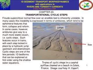
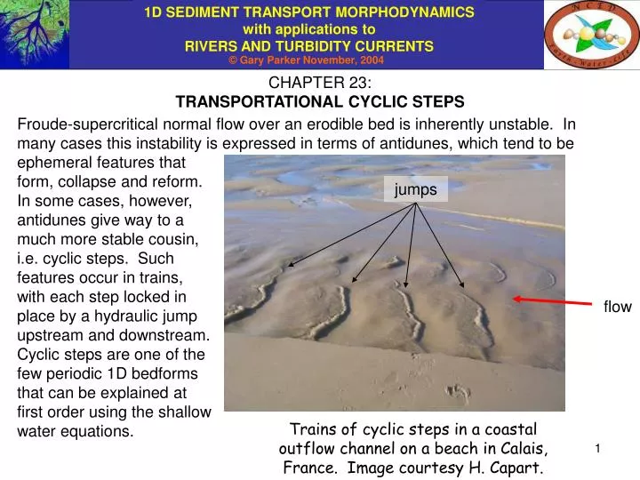
CHAPTER 23: TRANSPORTATIONAL CYCLIC STEPS. Froude-supercritical normal flow over an erodible bed is inherently unstable. In many cases this instability is expressed in terms of antidunes, which tend to be.

E N D
CHAPTER 23: TRANSPORTATIONAL CYCLIC STEPS Froude-supercritical normal flow over an erodible bed is inherently unstable. In many cases this instability is expressed in terms of antidunes, which tend to be ephemeral features that form, collapse and reform. In some cases, however, antidunes give way to a much more stable cousin, i.e. cyclic steps. Such features occur in trains, with each step locked in place by a hydraulic jump upstream and downstream. Cyclic steps are one of the few periodic 1D bedforms that can be explained at first order using the shallow water equations. jumps flow Trains of cyclic steps in a coastal outflow channel on a beach in Calais, France. Image courtesy H. Capart.
INTRODUCTION TO TRANSPORTATIONAL CYCLIC STEPS The first clear description of transportational cyclic steps is due to Winterwerp et al. (1992), who described their formation as water drains out of a polder on the verge of being closed, so forming steps in loose sand. Winterwerp et al. also developed a formulation for flow and sediment transport over these steps that has many of the elements of a morphodynamic model. The name “cyclic steps” was proposed by Taki and Parker (in press) and Sun and Parker (in press), who developed the first complete first-order morphodynamic model for cyclic steps. The cyclic steps in the image to the left are “transportational” in that they result from the differential transport of sediment over an alluvial bed, as described in the next slide. Cyclic steps can also form in a purely erosional setting. jumps Trains of cyclic steps in an outflow channel of a polder in the Netherlands that is in the process of being closed. Image courtesy M. de Groot.
MORPHODYNAMICS OF EQUILIBRIUM TRANSPORTATIONAL STEPS Consider the train of bedforms illustrated below. The bedforms have wavelength L, wave height and upstream migration speed c. Each bedform is bounded upstream and downstream by a hydraulic jump. The dominant mode of sediment transport is suspension. The slow flow just downstream of the jump causes net deposition, and the swift flow just upstream of the jump causes net erosion. As a result, it is possible for the train to migrate upstream without changing form, and with no net bed aggradation or degradation when averaged over one wavelength.
EQUILIBRIUM TRANSPORTATIONAL STEPS IN THE LABORATORY Taki and Parker (in press) illustrated the formation of equilibrium transportational cyclic steps in the laboratory. Each of the squares denotes 1 cm2. supercritical subcritical hydraulic jump zone reworked by upstream-migrating steps
one two three four EQUILIBRIUM TRANSPORTATIONAL STEPS IN THE LABORATORY contd. In a sufficiently long flume, Taki and Parker (in press) were able to form equilibrium trains of up to four successive steps. As each step migrates into the headbox of the flume, a new one forms at the downstream end.
TRANSPORTATIONAL CYCLIC STEPS CAN ALSO FORM IN ALLUVIUM UNDER NET-AGGRADATIONAL AND NET-DEGRADATIONAL CONDITIONS. The video clip below documents cyclic steps on an experimental alluvial fan-delta undergoing first degradation due to base level fall, and then aggradation due to base level rise. The video has been speeded up by a factor of 360. Double-click to view. Video clip courtesy N. Strong, B. Sheets, W. Kim and C. Paola (Strong et al., in press) The steps are manifested as trains of upstream-migrating hydraulic jumps. rte-bookstepsfan.mpg: to run without relinking, download to same folder as PowerPoint presentations.
CYCLIC STEPS CAN ALSO FORM IN A PURELY EROSIONAL SETTING Reid (1989) has documented trains of erosional steps in discontinuous gullies. Similar purely erosional steps have been observed in bedrock (Wohl and Grodek, 1994)). Parker and Izumi (2000) have developed a theory for purely erosional cyclic steps. Train of bedrock steps on Gough Island, South Atlantic Ocean. Train of erosional steps in a gully in California. Adapted from Reid (1989).
EROSIONAL CYCLIC STEPS The hydraulic jumps of erosional cyclic steps can eventually evolve into a train of plunge pools (Brooks, xxxx). Double-click on the video (right) to see steps form in a simulated bedrock made with silica flour and kaolinite. Train of plunge pools in a bedrock stream in California. Image courtesy of M. Neumann. rte-bookbedrocksteps.mpg: to run without relinking, download to same folder as PowerPoint presentations.
EROSIONAL CYCLIC STEPS IN A MODEL DRAINAGE BASIN Hasbargen and Paola (2000) have performed experiments on the formation of drainage basins due to rainfall on a sediment consisting of a mix of silica flour and kaolinite. Base level was lowered at a constant rate during the experiments. Erosional cyclic steps were often found to form spontaneously during the experiments. Double-click to view the video (courtesy L. Hasbargen and C. Paola). The video is speeded up considerably. The steps are mainfested as upstream-migrating headcuts. The steps formed even though base level was lowered a constant rate. rte-bookdrainagebasin.mpg: to run without relinking, download to same folder as PowerPoint presentations.
flow subcritical supercritical CONCEPT: THE HYDRAULIC JUMP The morphodynamics of cyclic steps is intimately tied to the mechanics of hydraulic jumps. The Froude number Fr = U2/(gH), where H denotes depth and U denotes depth-averaged flow velocity, was introduced in Chapter 5. In open channel flow, the transition from swift, shallow supercritical flow (Fr > 1) to tranquil, deep subcritical flow requires passage through the shock known as a hydraulic jump. A hydraulic jump in a flume is illustrated below.
CONCEPT: THE HYDRAULIC JUMP contd. Spillways are often designed so as to dissipate energy by means of a hydraulic jump. The images below are from the upper St. Anthony Falls on the Mississippi River, Minneapolis, Minnesota USA.
CONJUGATE DEPTH RELATION FOR THE HYDRAULIC JUMP The illustrated channel below carries constant water discharge Q in a wide, rectangular channel of constant width B. The flow makes the transition from supercritical to subcritical through a hydraulic jump. Let the values of H and U just upstream of the hydraulic jump be denoted as Hu and Uu, and the corresponding values just downstream of the jump be denoted as Hd and Ud. Momentum balance in the illustrated control volume is considered (width B out of the page).
CONJUGATE DEPTH RELATION FOR THE HYDRAULIC JUMP contd. The control volume is assumed to be short enough to allow for the neglect of bed friction. The momentum discharge Qm and pressure force Fp were introduced in Chapter 5; Applying balance of streamwise momentum to a steady flow in the control volume below, the following relation is obtained.
CONJUGATE DEPTH RELATION FOR THE HYDRAULIC JUMP contd. Momentum balance thus yields the relation: The relation for water conservation is where Q denotes the constant water discharge, B denotes the (constant) width and qw denotes the (constant) water discharge per unit width. Now denoting = Hd/Hu and Fru2 = Uu2/(gHu) = qw2/(gHu3), the above two equations can be reduced to the form The only physically realistic roots to the polynomial are = 1 (no jump) and the conjugate depth relation for a hydraulic jump:
CONJUGATE DEPTH RELATION FOR THE HYDRAULIC JUMP contd. In so far as a) according to flow continuity qw = UH and b) the Froude number Fr is given as Fr = U2/(gH) = qw2/(gH3), the conjugate depth relation can be used to find the relation between the upstream and downstream (conjugate) flow velocities and Froude numbers: A hydraulic jump thus entails an increase in depth and decrease in velocity as the flow makes the transition from supercritical (Fru > 1) to subcritical (Frd < 1).
EQUILIBRIUM CYCLIC STEPS AS A PERMANENT PERIODIC WAVE TRAIN The experiments of Taki and Parker (in press) indicate that cyclic steps can reach an equilibrium state at which a periodic wave train migrates upstream without changing form. When this state is reached, average bed slope Se, wavelength L, wave height and wave migration speed c attain constant values. In this simplest of cases the morphodynamic problem reduces a search for a solution of permanent form. That is, the deviation of bed elevation d(x, t) from the line of equilibrium slope becomes a function of spatial coordinate alone when transformed to a coordinate system moving upstream with constant speed c. More precisely,
PARAMETERS • The analysis given here is based on that of Sun and Parker (in press), which captures the essential features of the experimental cyclic steps described in Taki and Parker (in press). The flow is treated as suspension-dominated, and bedload transport is neglected. The suspension is characterized with a single sediment size. • The following parameters are used in this chapter. • x = streamwise coordinate [L] t = time [T] • = bed elevation [L] H = flow depth [L] U = depth-averaged flow velocity [L/T] L = step wavelength [L] C = depth-averaged susp. sed conc. [1] c = upstream step migration speed [1] qw = water discharge per unit width [L2/T] g = gravitational acceleration [L/T2] Cf = bed friction coefficient [1] vs = fall velocity of susp. sed. [L/T] • = water density [M/L3] s = sediment density [M/L3] R = (s/ - 1) L = step wavelength [L] c = upstream migration speed of step [L/T] Se = mean equilibrium bed slope [1] b = CfU2 = bed shear stress [M/L/T2] p = bed porosity D = grain size [L] E = dimensionless rate of entrainment of bed sediment into suspension [1] = ratio of near bed concentration of suspended sediment to depth- averaged value [1]
GOVERNING EQUATIONS The governing equations for momentum and mass balance of the flow in a channel of constant width were derived in Chapter 5. They are as follows; The Exner equation of conservation of bed sediment was derived in Chapter 4. Upon the neglect of bedload transport, it takes the form where denotes the near-bed volume concentration of suspended sediment. The equation of conservation of sediment in suspension was also derived in Chapter 4. Neglecting bedload transport, it takes the form deposition entrainment entrainment deposition
REDUCTION OF THE RELATIONS FOR SEDIMENT CONSERVATION The following assumptions are introduced to close the equations of conservation of bed sediment and sediment in suspension; where ro and c are (for most cases of interest) order-one parameters. The first of these assumptions was introduced in Chapter 21. The material of Chapter 10 (Slides 21-25 and the condition E = ) can be used to derive quasi-equilibrium forms for ro and c; In the present analysis ro and c are approximated as constants. It is easily demonstrated that ro and c tend toward unity as vs/u* approaches 0.
REDUCTION contd With the assumptions of the previous slide, the following approximate shallow-water forms are used to treat the case of cyclic steps: In the case of the experiments of Taki and Parker (in press), the suspensions were sufficiently vigorous that the assumptions ro = c = 1 could be applied. These assumptions are also used here. The analysis easily generalizes, however, to the range for which ro and c are not equal to unity.
MOBILE-BED EQUILIBRIUM IN THE ABSENCE OF STEPS An equilibrium solution can always be found for the case of a constant flow over a constant slope in the absence of steps. In the range where steps form, this equilibrium without steps is unstable, and devolves to a new equilibrium with steps. Having said this, however, it is useful to characterize the equilibrium solution without steps before proceeding with the analysis. Let Sn, Hn, Un, Cn, En and qsn denote equilibrium values of S, H, U, C, E and qs = UHC in the absence of steps. Where qw denotes constant water discharge per unit width, Cfeed denotes the constant volume feed concentration of sediment and Cf denotes the bed friction coefficient (here assumed to be constant for simplicity), the governing equations reduce to the following equilibrium forms:
FRICTION COEFFICIENT IN THE ABSENCE OF STEPS Taki and Parker (in press) used data from their experiments pertaining to equilibrium without steps to evaluate Cf and E in the absence of steps. They used three grades of silica flour, with nominal sizes of 19, 45 and 120 m. Within the scatter of the data, the friction coefficient was found to be roughly constant, as shown below. Note that D denotes grain size. H/D
SEDIMENT ENTRAINMENT IN THE ABSENCE OF STEPS In the experiments of Taki and Parker (in press), the flow was only a few mm thick, and no existing relation for the entrainment rate E could be used. With this in mind, they used data for the case of equilibrium without steps to determine a relation of the general form of van Rijn (1984); where denotes the kinematic viscosity of water, In the above relations and Ut denotes a critical velocity for the entrainment of bed sediment into suspension. The above relations reduce to the form
EVALUATION OF THE SEDIMENT ENTRAINMENT RELATION The scatter in the data was sufficient to allow the fitting of a relation with exponents in the range 1.5 n 2.5. The fit using the exponent of 2.0 is shown below. E/t
EVALUATION OF THE SEDIMENT ENTRAINMENT RELATION contd The fits of t and th* versus Rep to the data of Taki and Parker (in press) are given below for the cases n = 1.5, 2.0 and 2.5. The reference “Mantz” pertains to experiments due Mantz (1977) on the threshold of motion for fine particles.
National Center for Earth-surface Dynamics Our vision: Integrated, predictive science of the processes and interactions that shape the Earth’s surface CALCULATION OF MOBILE-BED EQUILIBRIUM WITHOUT STEPS In many of the experiments of Taki and Parker (in press), steps formed only after the establishment of a mobile-bed equilibrium without steps. Such an equilibrium is shown below. flow The flume is 10 cm wide and either 2 or 4 m long. The flow is only a few mm deep.
CALCULATION OF MOBILE-BED EQUILIBRIUM WITHOUT STEPS contd The results and relations used in the previous slides can be used to “predict” the mobile-bed equilibrium state without steps. Let D, R, , qw, Cfeed and Cf be specified, and let n be chosen (e.g. n = 2.0). Rep is computed from the first three of these parameters, and t and th* are then computed from the diagram of Slide 25. The parameter Uth is computed from the relation Since according to Slide 21 E = Cfeed for this state, flow velocity Un in the absence of steps is computed from the relation The flow depth Hn and bed slope Sn in the absence of steps are computed from The latter relation can be rearranged to the form where Frn denotes the Froude number at mobile-bed equilibrium without steps.
RANGE OF INTEREST; EQUILIBRIUM AT THRESHOLD STATE Taki and Parker (in press) found that cyclic steps would form only when the mobile-bed equilibrium flow without steps was supercritical. The range of interest is, then, It will also prove of interest here to examine the equilibrium state at the threshold of motion that prevails for the same values of D, R, , qw and Cf as in the case of mobile-bed equilibrium, but with vanishing values of Cfeed and qsn. Let Ht, St, Ut and Frt be the values of H, U, S and Froude number Fr at the threshold of motion.
EQUILIBRIUM AT THRESHOLD STATE contd The threshold state is of interest for the following reason. When steps form, they are accompanied by hydraulic jumps. It is reasonable to assume that the bed shear stress b just after the hydraulic jump is reduced to the threshold value for the entrainment of sediment. Recall that D, R, , qw and Cf take the same values as in the case of mobile-bed equilibrium. The method of computation of th* and Ut has already been outlined in Slide 27. The values of Ht, St and Froude number Frt are computed from the relations In so far as it is speculated that threshold conditions are realized just after the hydraulic jump (where by definition the flow must be subcritical, the range of interest is then Threshold of motion attained here?
FORMULATION IN THE PRESENCE OF STEPS • The following simplifying assumptions are made to treat the case for which cyclic steps are present. • The friction coefficient Cf takes the same value as it does at mobile-bed equilibrium without steps. • The entrainment relation evaluated at mobile-bed equilibrium without steps can be generalized to the the case for which steps are present, so that where U denotes the local flow velocity, the local entrainment rate is given as The appropriate balance relations are taken to be those of Slide 20 (but with ro = c = 1).
EQUILIBRIUM STEPS: TRANSFORMATION TO MOVING COORDINATES The solution sought here is one of permanent form: the steps migrate upstream at constant speed c without changing form, and without net aggradation or degradation averaged over one wavelength. Let Se denote the equilibrium average slope in the presence of steps, and let bed elevation be given as where u denotes an upstream bed elevation at x = 0 and d denotes the deviatoric bed elevation associated with the steps.
EQUILIBRIUM STEPS: TRANFORMATION TO MOVING COORDINATES contd. The balance equations of Slide 20 are reduced with the assumptions ro = c = 1 and the relation of the previous slide to obtain the forms They are then transformed to coordinates moving upstream with speed c as
EQUILIBRIUM STEPS: TRANSFORMATION TO MOVING COORDINATES contd. The results of the transformation are For a solution of permanent form, all time derivatives /tm must vanish. In addition, in the experiments of Taki and Parker (in press), the following condition was satisfied:
RESULTS OF THE TRANSFORMATION After the coordinate transformation, neglect of the time derivatives and application of the condition c/U << 1, the following relations are obtained.
BOUNDARY CONDITIONS Recall that the wavelength of a step is denoted as L. According to the figure below, the boundary conditions on deviatoric bed elevation are The flow at xm = 0 is just after a hydraulic jump where it is assumed that threshold conditions are attained, and the flow at xm = L is just before a hydraulic jump. As a result, the boundary conditions on U are Threshold velocity Conjugate velocity See Slide 15
BOUNDARY CONDITIONS contd In order for the train of steps to be in equilibrium with the sediment supply, the transport rate of suspended sediment averaged over the steps must be equal to the feed rate. Thus the transport rate qs = UHC = qwC averaged over one wavelength must equal the feed rate qwCfeed: Upon reduction, then,
REDUCTION AND NON-DIMENSIONALIZATION The following equations of Slide 34 reduce to a form of the backwater equation involving flow velocity; The above equation and the relations of sediment conservation of Slide 34, i.e. are made dimensionless using the following transformations;
NON-DIMENSIONALIZATION contd When placed in non-dimensional form and reduced with the relation CfFrt2 = St of Slide 29, the following relations result: where dimensionless wave speed, sediment fall velocity and bed slope and normalized entrainment rate are given as In addition, dimensionless wavelength is given as
NON-DIMENSIONALIZATION contd The dimensionless forms for the boundary conditions are The normalized entrainment rate can be reduced with the forms on Slides 27 and 30 to the form and Un is the flow velocity at the mobile-bed equilibrium state discussed in Slides 26 and 27.
REDUCTION OF DIMENSIONLESS FORMS The normalized entrainment rate can be further reduced with the definitions to the form
REDUCTION OF DIMENSIONLESS FORMS contd Substituting into results in the form Between and it is found that Applying the boundary conditions yields the results Suspended sediment concentration is continuous through the hydraulic jump.
FINAL FORM OF THE PROBLEM Solve where subject to the boundary conditions The problem consists of two first-order ordinary differential equations subject to four boundary conditions.
CHARACTER OF THE PROBLEM: SINGULARITY The problem defines an overspecified system of ordinary differential equations. That is; a) There are 2 first-order differential equations in and , b) plus the 4 parameters Frt, Frn, Sr and , c) Subject to 4 boundary conditions. Thus if any two of Frt, Frn, Sr and are specified, , and the other two parameters can be computed. Note, however, that the equation for becomes singular when the denominator on the right-hand side vanishes. The problem cannot be solved without overcoming this singularity.
NATURE OF THE SINGULARITY Now at the singularity or thus Just after the hydraulic jump, the flow is subcritical. As the flow progresses from left to right, it must pass through a Froude number Fr of unity at some point and become supercritical. The equation blows up as the flow passes from subcritical to supercritical. Image courtesy J. White
REMOVAL OF THE SINGULARITY: L’HOPITAL’S RULE The denominator of the right-hand side of the equation vanishes at where . Thus in order to avoid singular behavior the numerator of the right-hand side must also vanish, yielding the relation Here the subscript “1” denotes the value at . Reducing the this relation with the relation given above for and the evaluation of of Slide 40, it is found that
REMOVAL OF THE SINGULARITY: L’HOPITAL’S RULE contd Now at the equation in question takes the form Applying L’hopital’s rule at , Now denoting , after some algebra it is found that where
SOLUTION PROCEDURE • The parameter must be specified in advance. • Specify values of Frn and Frt. • Guess solutions for Sr and . • Define the variable • Integrate the following two equations upstream to the point where • (threshold condition). • The conditions on these equations at are
SOLUTION PROCEDURE contd • Integrate the same two equations i.e. • subject to the same conditions at , downstream to , where • For every guessed pair the dimensionless wavelength is then given as • The resulting solutions for and take the forms
SOLUTION PROCEDURE contd • The remaining two boundary conditions are • or • For specified values of Frt and Frn, the correct values of and Sr are the ones that satisfy the above equations. These values must be found iteratively. Both the bisection and Newton-Raphson iterative techniques have been found to yield solutions. • In the material presented subsequently the bisection method has been used. Details are presented in Sun and Parker (in press).
PREDICTED AND OBSERVED REGION OF FORMATION OF STEPS, 19 m SEDIMENT The solid lines enclose the region within which cyclic steps are predicted by Sun and Parker (in press). The points (M or S) are observed values from Taki and Parker. Here “M” denotes the fact that a train of multiple steps was observed, whereas “S” denotes the fact that a single step was observed.