Download
1 / 78
780 likes | 866 Views
Price Elasticity of Demand. Overheads. A Little Photo Retrospective. Malcolm X. Paul McCartney. Sidney Poitier. Howard Cossel. Bill Cosby. Joe Frazier. Joe Lewis. Jackson 5. Nelson Mandela. How much would your roommate pay to watch a live fight?. How does Showtime decide how

E N D
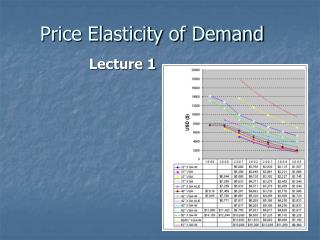
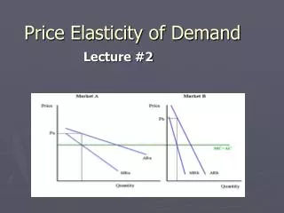
Price Elasticity of Demand Overheads
A Little Photo Retrospective Malcolm X Paul McCartney
Sidney Poitier Howard Cossel
Bill Cosby Joe Frazier
Joe Lewis Jackson 5
How much would your roommate pay to watch a live fight? How does Showtime decide how much to charge for a live fight?
What about Hank and Son’s Concrete? How much should they charge per square foot? Can ISU raise parking revenue by raising parking fees? Or will the increase in price drive demand down so far that revenue falls?
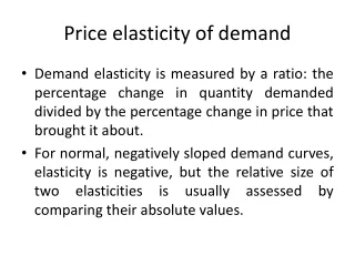
All of these pricing issues revolve around the issue of how responsive the quantity demanded is to price. Elasticity is a measure of how responsive one variable is to changes in another variable?
The Law of Demand The law of demand states that when the price of a good rises, and everything else remains the same, the quantity of the good demanded will fall. The real issue is how far it will fall.
The demand function is given by QD = quantity demanded P = price of the good ZD = other factors that affect demand
The inverse demand function is given by To obtain the inverse demand function we just solve the demand function for P as a function of Q
Examples QD = 20 - 2P 2P + QD = 20 2P = 20 - QD P = 10 - 1/2 QD Slope = - 1/2
Examples QD = 60 - 3P 3P + QD = 60 3P = 60 - QD P = 20 - 1/3 QD Slope = - 1/3
One measure of responsiveness is slope For demand The slope of a demand curve is given by the change in Q divided by the change in P
For inverse demand The slope of an inverse demand curve is given by the change in P divided by the change in Q
Examples QD = 60 - 3P Slope = - 3 P = 20 - 1/3 QD Slope = - 1/3
Examples QD = 20 - 2P Slope = - 2 P = 10 - 1/2 QD Slope = - 1/2
Q P We can also find slope from tabular data Q P 0 10 2 9 4 8 6 7 8 6 10 5
Demand for Handballs Q P 0 10 1 9.5 2 9 3 8.5 4 8 5 7.5 6 7 7 6.5 8 6 9 5.5 10 5 11 4.5 12 4 13 3.5 14 3 15 2.5 16 2 17 1.5 18 1 19 0.5 20 0
P Q P 0 10 1 9.5 2 9 3 8.5 4 8 5 7.5 6 7 7 6.5 8 6 9 5.5 10 5 11 4.5 12 4 13 3.5 14 3 15 2.5 16 2 17 1.5 18 1 19 0.5 20 0 Demand for Handballs 11 10 Price 9 8 7 6 5 4 3 2 1 0 0 2 4 6 8 10 12 14 16 18 20 22 Quantity
Q P Q P 0 10 1 9.5 2 9 3 8.5 4 8 5 7.5 6 7 7 6.5 8 6 9 5.5 10 5 11 4.5 12 4 13 3.5 14 3 15 2.5 16 2 17 1.5 18 1 19 0.5 20 0 Demand for Handballs 11 10 Price Q = 2 - 4 = -2 9 8 P = 9 - 8 = 1 7 6 5 4 3 2 1 0 0 2 4 6 8 10 12 14 16 18 20 22 Quantity
Problems with slope as a measure of responsiveness Slope depends on the units of measurement The same slope can be associated with very different percentage changes
Examples QD = 200 - 2P 2P + QD = 200 2P = 200 - QD P = 100 - 1/2 QD
P Q Q P 0 100 1 99.5 2 99 3 98.5 4 98 5 97.5 6 97 7 96.5 8 96 9 95.5 10 95 11 94.5 12 94 13 93.5 14 93 Consider data on racquets Let P change from 95 to 96 P = 96 - 95 = 1 Q = 8 - 10 = -2 A $1.00 price change when P = $95.00 is tiny
Graphically for racquets Demand for Racquets 102 Price 100 98 96 Slope = - 1/2 94 92 90 88 0 2 4 6 8 10 12 14 16 18 Large % change in Q Quantity Small % change in P
Graphically for hand balls Demand for Handballs 11 10 Price P = 7 - 6 = 1 9 8 7 6 Q = 6 - 8 = -2 P 5 4 3 Slope = - 1/2 2 1 0 0 2 4 6 8 10 12 14 16 18 20 22 Quantity Large % change in Q Large % change in P
So slope is not such a good measure of responsiveness Instead of slope we use percentage changes The ratio of the percentage change in one variable to the percentage change in another variable is called elasticity
The Own Price Elasticity of Demand is given by There are a number of ways to compute percentage changes
Initial point method for computing The Own Price Elasticity of Demand
Q P Price Elasticity of Demand (Initial Point Method) P Q 6 8 5.5 9 5 10 4.5 11 4 12
Final point method for computing The Own Price Elasticity of Demand
Q P Price Elasticity of Demand (Final Point Method) P Q 6 8 5.5 9 5 10 4.5 11 4 12
The answer is very different depending on the choice of the base point So we usually use The midpoint method for computing The Own Price Elasticity of Demand
Elasticity of Demand Using the Mid-Point For QD we use the midpoint of the Q’s
Similarly for prices For P we use the midpoint of the P’s
Price Elasticity of Demand (Mid-Point Method) Q P 8 6 9 5.5 10 5 11 4.5 12 4
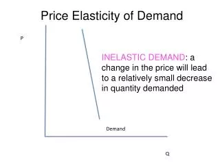
Classification of the elasticity of demand Inelastic demand When the numerical value of the elasticity of demand is between 0 and -1.0, we say that demand is inelastic.
Classification of the elasticity of demand Elastic demand When the numerical value of the elasticity of demand is less than -1.0, we say that demand is elastic.
Classification of the elasticity of demand Unitary elastic demand When the numerical value of the elasticity of demand is equal to -1.0, we say that demand is unitary elastic.
Classification of the elasticity of demand Perfectly elastic - D = - horizontal Perfectly inelastic - D = 0 vertical
Elasticity of demand with linear demand Consider a linear inverse demand function The slope is (-B) for all values of P and Q For example, The slope is -0.5 = - 1/2
Q Q P P P Q 12 0 11.5 1 11 2 10.5 3 10 4 9.5 5 9 6 8.5 7 8 8 7.5 9 7 10 6.5 11 6 12 5.5 13 5 14 4.5 15 4 16 3.5 17 3 18 Demand for Diskettes 13 12 Price 11 10 9 8 7 6 5 4 3 2 1 0 0 2 4 6 8 10 12 14 16 18 20 22 Quantity
Q P The slope is constant but the elasticity of demand will vary P Q 12 0 11.5 1 11 2 10.5 3 10 4 9.5 5 9 6 8.5 7 8 8 7.5 9 7 10 6.5 11 6 12 5.5 13 5 14 4.5 15 4 16 3.5 17 3 18
Q P The slope is constant but the elasticity of demand will vary P Q 12 0 11.5 1 11 2 10.5 3 10 4 9.5 5 9 6 8.5 7 8 8 7.5 9 7 10 6.5 11 6 12 5.5 13 5 14 4.5 15 4 16 3.5 17 3 18
P smaller Q larger The slope is constant but the elasticity of demand will vary A linear demand curve becomes more inelastic as we lower price and increase quantity The elasticity gets closer to zero
The slope is constant but the elasticity of demand will vary Q P Elasticity Expenditure 0 12 0 2 11 -23.0000 22 4 10 -7.0000 40 6 9 -3.8000 54 8 8 -2.4286 64 10 7 -1.6667 70 12 6 -1.1818 72 14 5 -0.8462 70 16 4 -0.6000 64 18 3 -0.4118 54 20 2 -0.2632 40 22 1 -0.1429 22 24 0 -0.0435 0
The slope is constant but the elasticity of demand will vary Q P Elasticity Expenditure 0 12 0 2 11 -23.0000 22 4 10 -7.0000 40 6 9 -3.8000 54 8 8 -2.4286 64 10 7 -1.6667 70 12 6 -1.1818 72 14 5 -0.8462 70 16 4 -0.6000 64 18 3 -0.4118 54 20 2 -0.2632 40 22 1 -0.1429 22 24 0 -0.0435 0