Download
1 / 40
400 likes | 502 Views
What Impact will Increased Commodity Prices Have on Land Values?. Rising Food and Energy Cost Conference Oregon State University October 2, 2008 John B. Penson, Jr. Regents Professor and Stiles Professor of Agriculture Texas A&M University. Factors Affecting Land Values.

E N D
What Impact will Increased Commodity Prices Have on Land Values? Rising Food and Energy Cost Conference Oregon State University October 2, 2008 John B. Penson, Jr. Regents Professor and Stiles Professor of Agriculture Texas A&M University
Factors Affecting Land Values • Expected future commodity prices. • Expected productivity and future cost of production inputs like fertilizer and seed. • Expected future interest rates. • Expected future land appreciation. • Income and capital gains tax rates. • Attitude toward risk and risk premium used when discounting annual cash flows.
Land values started falling in late 1979. Farm debt continued to expand well into 1982. Today’s boom Source: NASS - USDA. Real net farm income in 1983 virtually identical to 1933.
Average Value of Cropland by Farm Production Region Source: NASS - USDA
Markets studied today Source: NASS-USDA
Growth in global food demand. Russian wheat deal in 1972. Export expansion, low stocks. Tight world stocks, supply. Asian financial crisis in 97/98. Source: Iowa State University Extension Service. Rising crop prices. Growth in emerging countries. Growth in renewable fuels. Global recession. Fighting inflation. Strong dollar.
Average Cash Rent by Farm Production Region Source: NASS – USDA.
Markets studied today Source: NASS-USDA
Catch up time? Rents fell during financial crisis in the 1980s. Source: Chicago Federal Reserve District (IL, IA, MI, IN, WI); Chicago Federal Reserve District Bank.
A Practical Example • Assume that operating expenses for an Illinois corn farmer are $500 an acre as a result of rising fertilizer and seed prices. • Assume producer achieves a yield of 200 bushels an acre. • If cash rents are $300 an acre, the producer would need to receive $4.00 per bushel just to break even. • This would leave nothing for profit, debt payment coverage and family living expenses.
Source: Derived from Farm Sector Balance Sheet and Income Statements published by ERS – USDA.
Importance of government payments in 1980s crisis Source: Derived from Farm Sector Balance Sheet and Income Statements published by ERS – USDA.
Heart of farm financial crisis Source: Derived from Farm Sector Balance Sheet and Income Statements published by ERS – USDA.
A questionable USDA concept given that only one third of farmers have term debt!
Uncertainty in Capital Markets • Capital markets in disarray. • Commercial paper market seized up. • Libor rates up markedly. • 10 million home mortgages today have negative equity. Housing prices fell 17% in last twelve months. Bottom of housing market not yet in sight. • 40 percent of mortgages made in last two years were sub-prime loans. • 117 banks on FDIC trouble list in 2nd quarter.
Uncertainty in Real Economy • Institute of Supply Management business activity index fell to lowest level (43.5) since October 2001. Value below 50 signals business contraction. • Real wages sliding since November 2003; down sharply since August 2007. • Contagious effects on client nations for agricultural products, leading to declining exports. • Incomes declined for first time since August 2005. • Consumer spending adjusted for inflation at the lowest level in four years.
Recession Prospects • There can be no doubt that the U.S. economy is in a recession. • The question is how long it will last and how deep it will be. • I think it will be 1-2 years given passage of the bailout package passed and signed. • May look much like the 1981-1982 recession that lasted 16 months. • We know what that agriculture looked like during that recession.
Expansion of corn use in manufacturing ethanol comes at expense of feed use and has driven up corn prices. Source: Various WASDE Reports, USDA.
Instability in input prices as well Source: Agricultural Prices, NASS-USDA.
Source: 2007 expenses derived from published state crop production budgets. Projections over the 2008-2014 period based upon the rate of increase in FAPRI-Missouri projections updated in August 2008 extrapolated to 2017.
Source: Historical data for 1987-2007 provided by NASS-USDA. Projections for the 2008-2017 obtained from FAPRI-Missouri (2008-2013) updated in August 2008 and FAPRI-Iowa State (2014-2017).
Simulation Assumptions • Land values are local; reflect expected returns. • Focus on the capitalized agricultural value. • Net present value of future values over the 2008-2017 period; solution for maximum bid price or where price results in NPV=0. • Three crop situations examined: • Northern Central Kansas 65 bushel wheat • Iowa 170 bushel continuous corn • Central Illinois 182 bushel continuous corn
Scenario Design • Baseline – FAPRI commodity price and expense trends. • 15% higher commodity prices with baseline expenses and existing interest rates (HP-BEXP). This is the Best Case Scenario. • Baseline commodity prices and 10% higher expenses, including higher interest rates (BP-HEXP). • Lower commodity prices and baseline expenses and interest rates (LP-BEXP). • 15% higher commodity prices and 10% higher expenses, including higher interest rates (HP-HEXP). • 15% lower commodity prices and 10% higher expenses and interest rates (LP-HEXP). This is the Worst Case Scenario.
The capitalization of future operations over a 10-year period approximates the 2007 land prices for continuous wheat in Kansas and continuous corn in both Iowa and Illinois.
HP-BEXP = 15% higher annual commodity prices; baseline expenses. BP-HEXP = baseline commodity prices; 10% higher expenses. LP-BEXP = 15% lower annual commodity prices; higher expenses. HP-HEXP = 15% higher commodity prices; 10% higher expenses. LP-HEXP = 15% lower commodity prices; 10% higher expenses.
HP-BEXP = 15% higher annual commodity prices; baseline expenses. BP-HEXP = baseline commodity prices; 10% higher expenses. LP-BEXP = 15% lower annual commodity prices; higher expenses. HP-HEXP = 15% higher commodity prices; 10% higher expenses. LP-HEXP = 15% lower commodity prices; 10% higher expenses.
Analysis of Results • Addressing the title given to me for my paper, land prices would increase markedly if higher commodity prices are expected over the next ten years, particularly in Kansas. • Conversely, land prices in Kansas are more vulnerable to lower commodity prices and higher expenses than observed in Iowa and Illinois. • Higher expenses can be tolerated if commodity prices rise simultaneously. • Higher expenses absent of higher commodity prices could cause land values to fall sharply. • The lower commodity price scenario still left prices above target price levels under the 2008 farm bill.
Some Thoughts • If interest rates remained low, the dollar remained weak and corn stocks remain at pipeline level, commodity prices for corn and wheat would remain strong in the 2008/09 marketing year. • Continued volatility likely going forward. Long run projections by those presented in a baseline never reflect potential volatility. FAPRI addresses this using stochastic simulation examining 500 alternative scenarios. Their CDF suggests, for example, that there is a 10% chance the price of corn would fall below $3.00. • Crude oil prices, value of the dollar, energy policy and growth in emerging economies are the major drivers going forward.
Downside Risks • Lower crude oil prices affecting demand for corn as a feedstock. • Higher unit costs of crop production. • Higher interest rates. • Stronger dollar. • Slower economic growth in client nations resulting from contagious financial crisis. • Expanding production response in competitor nations.
Financial Implications • Real estate values represent 85% of farm balance sheets – represents a key factor to the financial health in the farm sector. • Farmers who refinanced debts with inflated land values as collateral in the 1970s faced severe problems when land values plummeted in the 1980s – surge in bankruptcies and rural bank closings. • Sales of 4-wheel tractors up 30% in 2008; farm debt expanding but not as fast as the 1970s. • Lenders will recognize weaknesses earlier due to less reliance on collateral lending.
Final Thoughts • The approach taken to assess today’s land prices in the locations addressed validated published prices for the three locations studied. • These cropland bid prices are sensitive to future expectations for commodity prices, unit input costs and interest rates. • Locations chosen were based upon the availability of updated crop production budgets – higher yields, more efficient operations and marketing strategies not reliant on spot market prices can justify higher bid prices for cropland.