Download
1 / 41
410 likes | 608 Views
Basic Enzo Algorithms. Greg Bryan (Columbia University) gbryan@astro.columbia.edu. Topics. Hydrodynamics PPM ZEUS AMR Timestepping Projection Flux correction Gravity Root grid Subgrids Particles Chemistry & Cooling Multispecies. I. Hydrodynamics.

E N D
Basic EnzoAlgorithms Greg Bryan (Columbia University) gbryan@astro.columbia.edu
Topics • Hydrodynamics • PPM • ZEUS • AMR • Timestepping • Projection • Flux correction • Gravity • Root grid • Subgrids • Particles • Chemistry & Cooling • Multispecies
Fluid Equations - grid::SolveHydroEquations Mass conservation Momentum conservation Energy conservation Ideal Gas EOS Self-gravity Field names: Density, Pressure, TotalEnergy, InternalEnergy, Velocity1, Velocity2, Velocity3
grid class: accessing the fields – grid.h • In grid class: • BaryonFields[] – array of pointers to each field • Fortran (row-major) ordering within each field • GridRank– dimensionality of problem • GridDimensions[]– dimensions of this grid • GridStartIndex[]– Index of first “active” cell (usually 3) • First (and last) three cells are ghost or boundary zones intDensNum= FindField(Density, FieldType, NumberOfBaryonFields); int Vel1Num = FindField(Velocity1, FieldType, NumberOfBaryonFields); for (k = GridStartIndex[2]; k <= GridEndIndex[2]; k++) { for (j = GridStartIndex[1]; j <= GridEndIndex[1]; j++) { for (i = GridStartIndex[0]; i <= GridEndIndex[0]; i++) { BaryonField[Vel1Num][GINDEX(i,j,k)] *= BaryonField[DensNum][GINDEX(I,j,k)]; } } }
Enzo file name convention • General C++ routines: • Routine name: EvolveLevel(…) • In file: EvolveLevel.C • One routine per file! • grid methods: • Routine name: grid::MyName(…) • In file: Grid_MyName.C • Fortran routines: • Routine name: intvar(…) • In file: intvar.src • .src is used because routine is fed first through C preprocessor
PPM Solver: grid::SolvePPM_DE • HydroMethod = 0 • PPM: e.g. mass conservation equation • Flux conservative form: • In discrete form: • How to compute mass flux? • Note: multi-dimensions handled by operating splitting • grid::xEulerSweep.C, grid::yEulerSweep.C, grid::zEulerSweep.C Mass flux across j+1/2 boundary
Grid::SolvePPM_DE // Update in x-direction for (k = 0; k < GridDimension[2]; k++) { if (this->xEulerSweep(k, NumberOfSubgrids, SubgridFluxes, GridGlobalStart, CellWidthTemp, GravityOn, NumberOfColours, colnum) == FAIL) { fprintf(stderr, "Error in xEulerSweep. k = %d\n", k); ENZO_FAIL(""); } } // ENDFOR k // Update in y-direction for (i = 0; i < GridDimension[0]; i++) { if (this->yEulerSweep(i, NumberOfSubgrids, SubgridFluxes, GridGlobalStart, CellWidthTemp, GravityOn, NumberOfColours, colnum) == FAIL) { fprintf(stderr, "Error in yEulerSweep. i = %d\n", i); ENZO_FAIL(""); } } // ENDFOR i
PPM: 1D hydro update: grid::xEulerSweep • Copy 2D slice out of cube • Compute pressure on slice (pgas2d) • Calculate diffusion/steepening coefficients (calcdiss) • Compute Left and Right states on each cell edge (inteuler) • Solve Reimann problem at each cell edge (twoshock) • Compute fluxes of conserved quantities at each cell edge (euler) • Save fluxes for future use • Return slice to cube
PPM: reconstruction: inteuler • Piecewise parabolic representation: • Coefficients (Dq and q6) computed with mean q and qL, qR. • For smooth flow (like shown above), this is fine, but can cause a problem for discontinuities (e.g. shocks) • qL, qRare modified to ensuremonotonicity (no newextrema) qL q qR
PPM: Godunov method: twoshock • To compute flux at cell boundary, take two initial constant states and then solve Riemann problem at interface • Given solution, can compute flux across boundary • Advantage: correctly satisfies jump conditions for shock rarefaction wave left state right state contact discontinuity shock
PPM: Godunov method: inteuler, twoshock • For PPM, compute left and right states by averaging over characteristic region (causal region for time step Dt) • Average left and right regions become constant regions to be feed into Riemann solver (twoshock).
PPM: Eulerian corrections: euler • Eulerian case more complicated because cell edge is fixed. • Characteristic region for fixed cell more complicated: • Note that solution is not known ahead of time so two-step procedure is used (see Collela & Woodward 1984 for details) SUPERSONIC CASE SUBSONIC CASE
Difficulty with very high Mach flows • PPM is flux conservative so natural variables are mass, momentum, total energy • Internal energy (e) computed from total energy (E): • Problem can arise in very high Mach flows when E >> e • e is difference between two large numbers • Not important for flow dynamics since p is negligible • But can cause problems if we want accurate temperatures since Tae
Dual Energy Formalism: grid::ComputePresureDualEnergyFormalism • Solution: Also evolve equation for internal energy: • Select energy to use depending on ratio e/E: • Select with DualEnergyFormalism = 1 • Use when v/cs> ~20 • Q: Why not just use e? • A: Equation for e is not in conservative form (source term). • Source term in internal energy equation causes diffusion
Zeus Solver: grid::ZeusSolver • Traditional finite difference method • Artificial viscosity (see Stone & Norman 1992) • HydroMethod = 2 • Source step: ZeusSource • Pressure (and gravity) update: • Artificial viscosity: • Compression heating:
Zeus Solver: grid::ZeusSolver • Transport step: Zeus_xTransport • Note conservative form (transport part preserves mass) • Note vj+1 is face-centered so is really at cell-edge, but density needs to be interpolated. Zeus uses an upwinded van Leer (linear) interpolation: • Similarly for momentum and energy (and y and z) • Zeus_yTransport, Zeus_zTransport e.g.
Zeus Solver: grid::ZeusSolver • PPM is more accurate, slower but Zeus is faster and more robust. • PPM often fails (“dnu < 0” error) when fast cooling generates large density gradients. • Try out new hydro solvers in Enzo 2.0! • Implementation differences with PPM: • Internal energy equation only • In code, TotalEnergy field is really internal energy (ugh!) • Velocities are face-centered • BaryonField[Vel1Num][GINDEX(i,j,k)] really “lives” at i-1/2
AMR: EvolveHierarchy • Root grid NxNxN, so Dx = DomainWidth/N • Level L defined so Dx = DomainWidth/(N2L) • Starting with level 0, grid advanced by Dt • Main loop of EvolveHierarchy looks (roughly) like this: • EvolveLevel does the heavy lifting
Time Step: grid::ComputeTimeStep • Timestep on level L is minimum of constraints over all level L grids: • + others (e.g. MHD, FLD, etc.) CourantSafetyFactor ParticleCourantSafetyFactor MaximumExpansionFactor
AMR: EvolveLevel • Levels advanced as follows: • Timesteps may not be integer ratios • (Diagram assumes Courant condition dominates and sound speed is constant so: dtaDx) • This algorithm is defined in EvolveLevel
Advance grids on level: EvolveLevel • The logic of EvolveLevel is given (roughly) as: Already talked about this. recursive Next, we’ll talk about these
BC’s: SetBoundaryConditions • Setting “ghost” zones around outside of domain • grid::SetExternalBoundaryValues • Choices: reflecting, outflow, inflow, periodic • Only applied to level 0 grids (except periodic) • Otherwise, two step procedure: • Interpolate ghost (boundary) zones from level L-1 grid • grid::InterpolateBoundaryFromParent • Linear interpolation in time (OldBaryonFields) • Spatial interpolation controlled by InterpolationMethod • SecondOrderA recommended, default (3D, linear in space, monotonic) • Copy ghost zones from sibling grids • grid::CheckForOverlapand grid::CopyZonesFromGrid
Projection: grid::ProjectSolutionToParentGrid • Structured AMR produces redundancy: • coarse and fine grids cover same region • Need to restore consistency • Correct coarse cells once grids have all reach the same time:
Flux Correction: grid::CorrectForRefinedFluxes • Mismatch of fluxes occurs around boundary of fine grids • Coarse cell just outside boundary used coarse fluxes but coarse cell inside used fine fluxes • Both fine and coarse fluxes saved from hydro solver Uncorrected coarse value Coarse flux across boundary Sum of fine fluxes Over 4 (in 3D) abutting fine cells
Rebuilding the Hierarchy: RebuildHierarchy • Need to check for cells needing more refinement Check for new grids on level 1 (and below) Check for new grids on Level 2 (and below) Check for new grids on Level 3 (and below)
Refinement Criteria – grid::SetFlaggingField • Many ways to flag cells for refinement • CellFlaggingMethod = • Then rectangular grids must be chosen to cover all flagged cells with minimum “waste” • Done with machine vision technique • Looks for edges (inflection points in number of flagged cells) • ProtoSubgrid class
Self-Gravity (SelfGravity = 1) • Solve Poisson equation • PrepareDensityField • BaryonField[Density] copied to GravitatingMassField • Particle mass is deposited in 8 nearest cells (CIC) • Particle position advanced by ½ step • DepositParticleMassField • Root grid (level 0): • Potential solved with FFT • ComputePotentialFieldLevelZero • Potential differenced to get acceleration • grid::ComputeAccelerationField
Self-Gravity • Subgrids: • Potential interpolated to boundary from parent • Grid::PreparePotentialField • Each subgrid then solves Poisson equation using multigrid • Grid::SolveForPotential • Note: this has two issues: • Interpolation errors on boundary can propagate to fine levels • Generally only an issue for steep potentials (point mass) • Ameliorated by having 6 ghost zones for gravity grid • Subgrids can have inconsistent potential gradients across boundary • Improved by copying new boundary conditions from sibilings and resolving the Poisson equation (PotentialIterations = 4 by default) • More accurate methods in development
Other Gravitational sources – grid::ComputeAccelerationFieldExternal • Can also add fixed potential: • UniformGravity – constant field • PointSourceGravity – single point source • ExternalGravity – NFW profile
N-body dynamics • Particles contribute mass to GravitatingMassField • Particles accelerated by AccelerationField • Interpolated from grid (from 8 nearest cells) • Particles advanced using leapfrog • grid::ComputeAccelerations • Particles stored in the locally most-refined grid • ParticlePosition, ParticleVelocity, ParticleMass • Tracer particles (massless) also available
Chemistry • Follows multiple species and solve rate equations • MultiSpecies = 1: H, H+, He, He+, He++, e- • MultiSpecies = 2: adds H2, H2+, H- • MultiSpecies = 3: adds D, D+ and HD • grid:SolveRateEquations • (or grid::SolveRateAndCoolEquationsif RadiativeCooling > 0) • Rate equations solved using backwards differencing formula (BDF) with sub-cycles to prevent > 10% changes • Works well as long as chemical timescale notreallyshort
Radiative Cooling – grid::SolveRadiativeCooling • RadiativeCooling = 1 • Two modes: • MultiSpecies = 0 • Equilibrium cooling table (reads file cool_rates.in) • Sub-cycles so that De < 10% in one cooling step • MultiSpecies > 1 • Computes cooling rate self-consistently from tracked-species • MetalCooling = 1: adds metal cooling from Glover & Jappsen (2007) • MetalCooling = 2: adds metal cooling from Raymond-Smith code • MetalCooling = 3: Cloudy Cooling table (Smith, Sigurdsson & Abel 2008) • RadiationFieldType > 0 • Add predefined radiative heating and ionization
Star Formation • Work in progress – many modes • StarParticleCreation > 0 • turns on and selects method (1-9) • For more details, see web page • StarParticleFeedback > 0 • Only valid for methods 1, 2, 7 and 8
More Physics in 2.0 • See talks tomorrow!
Q. What is that name all about anyway? • A. Source: Wikipedia