Relational Query Optimization

1. Relational Query Optimization Query Processing: Topic 2

2. Overview of Query Optimization • Plan:Tree of R.A. ops, with choice of alg for each op. • Each operator typically implemented using a `getnext’ interface: when an operator is asked for the next output tuple, it `pulls’ on its inputs and computes them. • This is the iterator model. • Two main issues: • For a given query, what plans are considered? • Algorithm to search plan space for cheapest (estimated) plan. • How is the cost of a plan estimated? • Ideally: Want to find best plan. Practically: Avoid worst plans!

3. Relational Algebra Equivalences • Allow us to choose different join orders and to `push’ selections and projections ahead of joins. • Selections: (Cascade) (Commute) • Projections: (Cascade) (Associative) • Joins: R (S T) (R S) T (Commute) (R S) (S R) R (S T) (T R) S • Show that:

4. More Equivalences • A projection commutes with a selection that only uses attributes retained by the projection. • Selection between attributes of the two arguments of a cross-product converts cross-product to a join. • A selection on just attributes of R commutes with R S. (i.e., (R S) (R) S ) • Similarly, if a projection follows a join R S, we can `push’ it by retaining only attributes of R (and S) that are needed for the join or are kept by the projection.

5. Highlights of System R Optimizer • Impact: • Most widely used currently; works well for < 10 joins. • Cost estimation: Approximate art at best. • Statistics, maintained in system catalogs, used to estimate cost of operations and result sizes. • Considers combination of CPU and I/O costs. • Plan Space: Too large, must be pruned. • Only the space of left-deep plans is considered. • Left-deep plans allow output of each operator to be pipelinedinto the next operator without storing it in a temporary relation. • Cartesian products avoided.

6. Schema for Examples Sailors (sid: integer, sname: string, rating: integer, age: real) Reserves (sid: integer, bid: integer, day: dates, rname: string) • Similar to old schema; rname added for variations. • Reserves: • Each tuple is 40 bytes long, 100 tuples per page, 1000 pages. • Sailors: • Each tuple is 50 bytes long, 80 tuples per page, 500 pages.

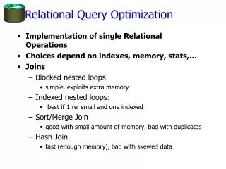
7. sname rating > 5 bid=100 sid=sid Sailors Reserves (On-the-fly) sname (On-the-fly) rating > 5 bid=100 (Simple Nested Loops) sid=sid Sailors Reserves RA Tree: Motivating Example SELECT S.sname FROM Reserves R, Sailors S WHERE R.sid=S.sid AND R.bid=100 AND S.rating>5 • Cost: 500+500*1000 I/Os • By no means the worst plan! • Misses several opportunities: selections could have been `pushed’ earlier, no use is made of any available indexes, etc. • Goal of optimization: To find more efficient plans that compute the same answer. Plan:

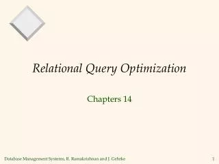
8. (On-the-fly) sname (Sort-Merge Join) sid=sid (Scan; (Scan; write to write to rating > 5 bid=100 temp T2) temp T1) Reserves Sailors Alternative Plans 1 (No Indexes) • Main difference: push selects. • With 5 buffers, cost of plan: • Scan Reserves (1000) + write temp T1 (10 pages, if we have 100 boats, uniform distribution). • Scan Sailors (500) + write temp T2 (250 pages, if we have 10 ratings). • Sort T1 (2*2*10), sort T2 (2*3*250), merge (10+250) • Total: 3560 page I/Os. • If we used BNL join, join cost = 10+4*250, total cost = 2770. • If we `push’ projections, T1 has only sid, T2 only sid and sname: • T1 fits in 3 pages, cost of BNL drops to under 250 pages, total < 2000.

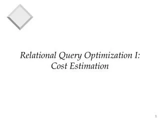
9. (On-the-fly) sname Alternative Plans 2With Indexes (On-the-fly) rating > 5 (Index Nested Loops, with pipelining ) sid=sid • With clustered index on bid of Reserves, we get 100,000/100 = 1000 tuples on 1000/100 = 10 pages. • INL with pipelining (outer is not materialized). (Use hash Sailors bid=100 index; do not write result to temp) Reserves • Projecting out unnecessary fields from outer doesn’t help. • Join column sid is a key for Sailors. • At most one matching tuple, unclustered index on sid OK. • Decision not to push rating>5 before the join is based on • availability of sid index on Sailors. • Cost: Selection of Reserves tuples (10 I/Os); for each, • must get matching Sailors tuple (1000*1.2); total 1210 I/Os.

10. Cost Estimation • For each plan considered, must estimate cost: • Must estimate costof each operation in plan tree. • Depends on input cardinalities. • We’ve already discussed how to estimate the cost of operations (sequential scan, index scan, joins, etc.) • Must estimate size of result for each operation in tree! • Use information about the input relations. • For selections and joins, assume independence of predicates. • We’ll discuss the System R cost estimation approach. • Very inexact, but works ok in practice. • More sophisticated techniques known now.

11. Statistics and Catalogs • Need information about the relations and indexes involved. Catalogstypically contain at least: • # tuples (NTuples) and # pages (NPages) for each relation. • # distinct key values (NKeys) and NPages for each index. • Index height, low/high key values (Low/High) for each tree index. • Catalogs updated periodically. • Updating whenever data changes is too expensive; lots of approximation anyway, so slight inconsistency ok. • More detailed information (e.g., histograms of the values in some field) are sometimes stored.

12. Size Estimation and Reduction Factors SELECT attribute list FROM relation list WHERE term1 AND ... ANDtermk • Consider a query block: • Maximum # tuples in result is the product of the cardinalities of relations in the FROM clause. • Reduction factor (RF) associated with eachtermreflects the impact of the term in reducing result size. Resultcardinality = Max # tuples * product of all RF’s. • Implicit assumption that terms are independent! • Term col=value has RF 1/NKeys(I), given index I on col • Term col1=col2 has RF 1/MAX(NKeys(I1), NKeys(I2)) • Term col>value has RF (High(I)-value)/(High(I)-Low(I))

13. Enumeration of Alternative Plans • There are two main cases: • Single-relation plans • Multiple-relation plans • For queries over a single relation, queries consist of a combination of selects, projects, and aggregate ops: • Each available access path (file scan / index) is considered, and the one with the least estimated cost is chosen. • The different operations are essentially carried out together (e.g., if an index is used for a selection, projection is done for each retrieved tuple, and the resulting tuples are pipelined into the aggregate computation).

14. Cost Estimates for Single-Relation Plans • Index I on primary key matches selection: • Cost is Height(I)+1 for a B+ tree, about 1.2 for hash index. • Clustered index I matching one or more selects: • (NPages(I)+NPages(R)) * product of RF’s of matching selects. • Non-clustered index I matching one or more selects: • (NPages(I)+NTuples(R)) * product of RF’s of matching selects. • Sequential scan of file: • NPages(R). • Note:Typically, no duplicate elimination on projections! (Exception: Done on answers if user says DISTINCT.)

15. Example SELECT S.sid FROM Sailors S WHERE S.rating=8 • If we have an index on rating: • (1/NKeys(I)) * NTuples(R) = (1/10) * 40000 tuples retrieved. • Clustered index: (1/NKeys(I)) * (NPages(I)+NPages(R)) = (1/10) * (50+500) pages are retrieved. (This is the cost.) • Unclustered index: (1/NKeys(I)) * (NPages(I)+NTuples(R)) = (1/10) * (50+40000) pages are retrieved. • If we have an index on sid: • Would have to retrieve all tuples/pages. With a clustered index, the cost is 50+500, with unclustered index, 50+40000. • Doing a file scan: • We retrieve all file pages (500).

16. D D C C D B A C B A B A Queries Over Multiple Relations • Fundamental decision in System R: only left-deep join treesare considered. • As the number of joins increases, the number of alternative plans grows rapidly; we need to restrict the search space. • Left-deep trees allow us to generate all fully pipelined plans. • Intermediate results not written to temporary files. • Not all left-deep trees are fully pipelined (e.g., SM join).

17. Enumeration of Left-Deep Plans • Left-deep plans differ only in the order of relations, the access method for each relation, and the join method for each join. • Enumerated using N passes (if N relations joined): • Pass 1: Find best 1-relation plan for each relation. • Pass 2: Find best way to join result of each 1-relation plan (as outer) to another relation. (All 2-relation plans.) • Pass N: Find best way to join result of a (N-1)-relation plan (as outer) to the N’th relation. (All N-relation plans.) • For each subset of relations, retain only: • Cheapest plan overall, plus • Cheapest plan for each interesting order of the tuples.

18. Enumeration of Plans (Contd.) • ORDER BY, GROUP BY, aggregates etc. handled as a final step, using either an `interestingly ordered’ plan or an addional sorting operator. • An N-1 way plan is not combined with an additional relation unless there is a join condition between them, unless all predicates in WHERE have been used up. • i.e., avoid Cartesian products if possible. • In spite of pruning plan space, this approach is still exponential in the # of tables.

19. Query Blocks: Units of Optimization SELECT S.sname FROM Sailors S WHERE S.age IN (SELECT MAX (S2.age) FROM Sailors S2 GROUP BY S2.rating) • An SQL query is parsed into a collection of queryblocks, and these are optimized one block at a time. • Nested blocks are usually treated as calls to a subroutine, made once per outer tuple. Outer block Nested block • For each block, the plans considered are: • All available access methods, for each reln in FROM clause. • All left-deep join trees(i.e., all ways to join the relations one-at-a-time, with the inner reln in the FROM clause, considering all reln permutations and join methods.)

20. SELECT S.sname FROM Sailors S WHERE EXISTS (SELECT * FROM Reserves R WHERE R.bid=103 AND R.sid=S.sid) Nested Queries • Nested block is optimized independently, with the outer tuple considered as providing a selection condition. • Outer block is optimized with the cost of `calling’ nested block computation taken into account. • Implicit ordering of these blocks means that some good strategies are not considered. The non-nested version of the query is typically optimized better. Nested block to optimize: SELECT * FROM Reserves R WHERE R.bid=103 AND S.sid= outer value Equivalent non-nested query: SELECT S.sname FROM Sailors S, Reserves R WHERE S.sid=R.sid AND R.bid=103

21. Summary • Query optimization is an important task in a relational DBMS. • Must understand optimization in order to understand the performance impact of a given database design (relations, indexes) on a workload (set of queries). • Two parts to optimizing a query: • Consider a set of alternative plans. • Must prune search space; typically, left-deep plans only. • Must estimate cost of each plan that is considered. • Must estimate size of result and cost for each plan node. • Key issues: Statistics, indexes, operator implementations.