Download
1 / 18
180 likes | 300 Views
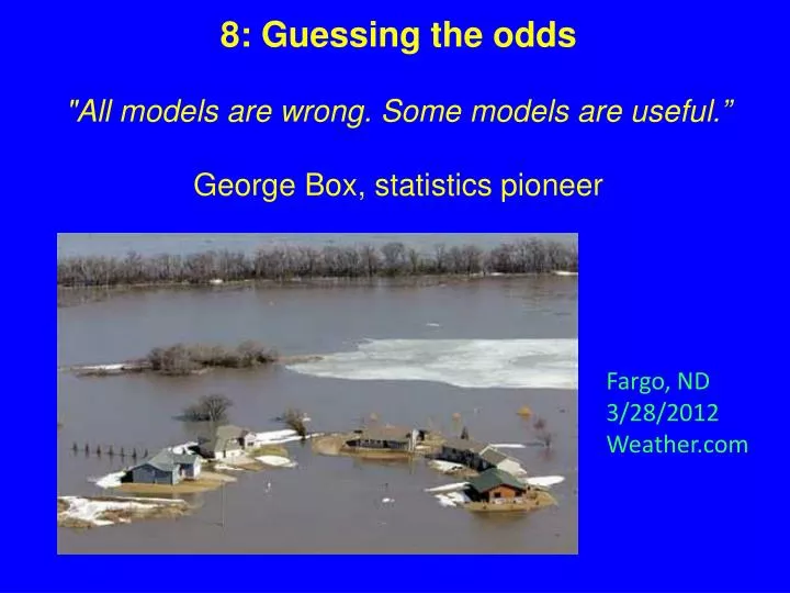
8: Guessing the odds "All models are wrong. Some models are useful .” George Box, statistics pioneer. Fargo, ND 3/28/2012 Weather.com. PAN 8.1: Estimation of flood frequency from a long-term record (Baer, SERC). 100 year flood. p – probability in 1 year = 1/100 = 0.01

E N D
8: Guessing the odds "All models are wrong. Some models are useful.” George Box, statistics pioneer Fargo, ND 3/28/2012 Weather.com
PAN 8.1: Estimation of flood frequency from a long-term record (Baer, SERC).
100 year flood p – probability in 1 year = 1/100 = 0.01 q – probability of not happening in 1 year = 1-p P(n,p) probability of at least 1 event in n years = 1 – probability of none = 1 – qn In 30 years P(30,p) = 0.26 = 26% In 100 years P(100,p) = 0.63 = 63% Contrary to our “intuition” P(n,p) is not equal to np (100 x 0.01 = 1) Lecture 8
PAN 8.2: Changes in flood frequency due to human activity (Dinicola, 1996).
PAN 8.3: A model for the probability of an event is drawing a ball from an urn filled with balls, some labeled "E" for event and others labeled "N" for none. (Stein and Stein, 2013a) Lecture 8
Time-independent probability If after we draw a ball we put it back in, successive draws are independent because the outcome of one does not change the probability of what will happen in the next. Put another way, the system has no “memory.” The joint probability P(AB) = P(A) P(B) Lecture 8
To estimate the probability of more than one event, we use the binomial probability distribution: giving the probability that in n trials there will be m events and (n − m) non-events. p and q are the probabilities of an event and a non-event. Cn,mis the number of ways we can have m events and n – m non-events, written in terms of factorials, where n! = n × (n − 1) × (n − 2) . . . × 3 × 2 × 1 and 0! = 1. For example, in three trials we can get one event and two non-events in C3,1 = 3!/(1!2!) = 3 ways: ENN, NEN, or NNE, so we multiply p1q2 by 3.
The binomial distribution is complicated to compute, so an approximation is used when the number of trials n is large and the probability p of an event is small. In this case, because n >> m and because p is small, we use a Taylor series These let us replace the binomial distribution by another probability distribution that is easier to compute, called a Poisson distribution
Poisson process used for time-independent probability If after we draw a ball we put it back in, successive draws are independent because the outcome of one does not change the probability of what will happen in the next. The system has no “memory,,” so events can’t be “overdue.” Lecture 8
CQ: Give an example you have encountered of the "gambler's fallacy" and explain why it was wrong.
Time-dependent probability We can add a number a of E-balls after a draw when an event does not occur, and remove r E-balls when an event occurs. This makes the probability of an event increase with time until one happens, after which it decreases and then grows again. Events are not independent, because one happening changes the probability of another.
PAN 8.4: Comparison of the probability of an event as a function of time for time-independent (solid line) and time-dependent (dashed lines) urn models. (Stein and Stein, 2013a) Lecture 8
PAN 8.5: Sequence of events as a function of time for the time-independent (top line) and time-dependent (lower lines) urn model runs in Figure 8.4. (Stein and Stein, 2013a) Lecture 8
http://www.telegraph.co.uk/topics/weather/9961052/Met-Office-ap...http://www.telegraph.co.uk/topics/weather/9961052/Met-Office-ap...
CQ: In March 2012, Britain's Meterological Office told the government "The forecast for average UK rainfall slightly favours drier than average conditions for April-May-June, and slightly favours April being the driest of the three months." Water companies prepared for water shortages. Later, the office admitted that "Given that April was the wettest since detailed records began in 1910 and the April-May-June quarter was also the wettest, this advice was not helpful.” Its chief scientist stated "The probabilistic forecast can be considered as somewhat like a form guide for a horse race. It provides an insight into which outcomes are most likely, although in some cases there is a broad spread of outcomes, analogous to a race in which there is no strong favourite. Just as any of the horses in the race could win the race, any of the outcomes could occur, but some are more likely than others." How do you respond to these statements? What - if anything - would you suggest doing differently?