An Immersed Boundary Method Enabling Large-Eddy Simulations of Complex Terrain in the WRF Model

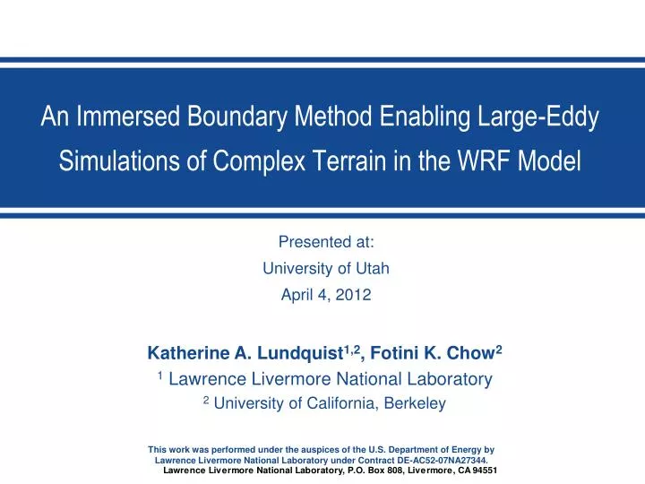
1. Performance Measures x.x, x.x, and x.x An Immersed Boundary Method Enabling Large-Eddy Simulations of Complex Terrain in the WRF Model Presented at: University of Utah April 4, 2012 Katherine A. Lundquist1,2, Fotini K. Chow2 1 Lawrence Livermore National Laboratory 2University of California, Berkeley

2. Numerical Weather Prediction in Complex Terrain Vertical coordinate systems used in numerical weather prediction models. orthogonal Non-orthogonal sigma, or terrain-following eta, or “step mountain”

3. Numerical Weather Prediction in Complex Terrain Nested grids used in mesoscale modelsallow integration of physical processes across a range of scales 1 km grid 300 m grid 50 m grid

4. Numerical Weather Prediction in Complex Terrain Higher grid resolution leads to steeper slopes in complex terrain

5. Problems with Terrain-Following Coordinates in Complex Terrain • Grid skewness leads to significant errors in horizontal derivatives • Advection • Diffusion • Pressure gradient Mapping function for coordinate transformation (Gal-Chen and Sommerville ,1975) New terms are introduced into the governing equations (metric terms) When discretized, the metric terms have additional truncation errors

6. Problems with Terrain-Following Coordinates in Complex Terrain In addition to truncation errors, numerical inconsistencies arise when: In the transformed coordinate η, the horizontal derivative is: Δz ht A first order finite difference approximation yields:

7. Problems with Terrain-Following Coordinates in Complex Terrain Numerically inconsistent derivatives are more likely at large aspect ratios Horizontal grid spacing of 1km with a vertical grid of 50 m leads to an aspect ratio of 20 • Moral of the story: Don’t stretch grids too much • Example: 1 km horizontal spacing, 50 m vertical -- max allowed slope is 3 degrees

8. How can we quantify numerical errors due to terrain-following coordinates? • Model fails at steep slopes, but when does solution quality deteriorate? • What slope? • What grid aspect ratio?

9. Numerical Weather Prediction in Complex Terrain Vertical coordinate systems used in numerical weather prediction models. orthogonal Non-orthogonal sigma, or terrain-following eta, or “step mountain” orthogonal • Use immersed boundary method • Can eliminate the terrain-following coordinate transformation • Quantify numerical errors through direct comparison of the two solutions immersed boundary

10. Scalar Advection Test Case (Schär et al. 2002) Domain Set-Up & Initialization • Peak Height = 3 km • Elevated Velocity Shear Layer at 5 km (terrain is very steep, but isolated) • Inviscid flow- no mixing • Stable Stratification • Domain size 300 km x 25 km • Grid spacing 1 km x 0.5 km • 5th order horizontal and 3rd order vertical advection scheme is used

11. Scalar Advection Test CaseGrid Configuration WRF Grid distortion IBM-WRF

12. Scalar Advection Test CaseVelocity Comparisons U (m/s) at t = 10000 s W (m/s) at t = 10000 s WRF WRF Height (km) IBM-WRF IBM-WRF Height (km) x (km) x (km)

13. Scalar Advection Test CaseScalar Concentration and Error

14. Error Terrain slope (degrees) Effects of terrain slope in WRF • Change max mountain height • Error = max(|WRF-exact|)

15. Atmosphere At Rest • 3D hill, quiescent atmosphere, no forcing • 10 degree slope (not very steep!) • Stable atmosphere • No flow should develop at all

16. Atmosphere at RestSpurious Flow Develops WRF horiz. diffusion WRF coord. diffusion IBM-WRF θ(K) θ(K) θ(K) U (m/s) U (m/s) U (m/s) Max velocity 3.8 e-5 m/s Max velocity 1.7 m/s Max velocity 0.28 m/s

17. Flow Over 3D Hill • Compare WRF and IBM-WRF • max slope of 10, 20, 30 deg, grid aspect ratio 1 • Geostrophic pressure gradient forcing • No-slip boundary condition • Zero flux condition on temperature • Run to steady state

18. Flow Over 3D HillVelocity Difference – WRF vs IBM-WRF Absolute velocity difference – slice through peak of hill 10 slope 20 slope 30 slope ht (km) x (km) x (km) x (km) Max u diff 1.0 m/s Max u diff 1.8 m/s Max u diff 3.1 m/s

19. Increased turbulent eddy viscosity • Overwhelms numerical errors • Absolute differences between WRF and IBM-WRF decrease Low viscosity High viscosity Height (km) x (km) x (km)

20. Immersed Boundary Method The immersed boundary method is a technique for representing boundaries on a non-conforming grid The effects of the body on the flow are represented by the addition of a forcing term in the momentum equation.

21. Immersed Boundary MethodFormulation of the Forcing Term • IBM was first used by Peskin (1972) and (1977) to simulate blood flow through the mitral valve of the heart. • Direct (or Discrete) Forcing proposed by Mohd-Yusof (1997) and used to model laminar flow over a ribbed channel Source: Peskin (1977) where VΩ is the desired Dirichlet boundary condition

22. Immersed Boundary MethodBoundary reconstruction Immersed Boundary Method grid Stair step or nearest neighbor grid Boundary is coincident with computational nodes Boundary effects must be interpolated to computational nodes

23. Immersed Boundary MethodBoundary Reconstruction Using a ghost cell method, the forcing term is applied within the solid domain. U2 U1 UΩ1 UΩ2 Ughost cell

24. Scalar Fluxes at the Immersed Boundary Use the immersed boundary method to impose boundary conditions on temperature, moisture, passive scalars, etc. A Dirichlet boundary condition Or a flux boundary condition can be imposed with IBM.

25. Immersed Boundary MethodBoundary Reconstruction Neumann boundary conditions are set by modifying the interpolation matrix to include the boundary condition Φ1 Φ2 δΦ/δnΩ1 δΦ/δnΩ2 Φghost cell

26. Idealized Valley Simulations • Thermal Slope flow induced by diurnal heating • Uncoupled simulations with specified surface heating • Coupled simulations using atmospheric parameterizations WARM

27. Idealized Valley Simulations Set-up and Initialization • ΔX = ΔY = 200 m, ΔZ ~100 m • (U,V,W) = (0,0,0) • Stable Potential Temp. • 40% Relative Humidity • Sandy Loam, Savannah • Soil Moisture, 20% saturation rate • Soil Temperature, equal to atmospheric temperature

28. Uncoupled Ideal Valley • Integrate from 6:00 to 18:00 UTC • Specified heat flux • Zero moisture flux at surface • No atmospheric physics • No surface properties • Constant

29. Uncoupled Ideal Valley Evolution of Potential Temp. Potential Temp at Valley Center

30. Coupled Ideal ValleyComparison of Velocity Profiles Comparison of instantaneous velocity profiles for IBM-WRF (red) and WRF (black)

31. Coupled Ideal Valley • Fully Coupled Model • RRTM Longwave Radiation • MM5 Shortwave Radiation • MM5 Surface Layer Model • NOAH Land Surface Model • Each atmospheric physics module has been modified to account for the immersed boundary

32. Coupled Ideal Valley Initialization • Date: March 21, 2007 • Location: 36°N, 0°E • Sandy Loam, Savannah • Soil Moisture, 20% saturation rate • Soil Temperature, equal to atmospheric temperature

33. Coupling IBM to the Atmospheric Physics Models • Surface physics models interact with the lowest coordinate level when terrain-following grids are used • The atmospheric physics models used here are column models • For radiation models the vertical integration limits are modified to exclude any portion of the atmosphere below the terrain • For surface physics a modified reference height is calculated and used with similarity theory

34. Coupled Ideal Valley Radiation Models Spatial variation in radiation at 12:00. Error from IBM coupling is negligible in comparison to changes with terrain height. Domain averaged incoming radiation (longwave and shortwave) differ by less than 0.43% during the simulation.

35. Coupled Ideal Valley Surface Physics Domain averaged heat flux differs by less than 5.4%, and moisture fluxes by less than 0.74%

36. Coupled Ideal ValleyLand-Surface Properties IBM provides boundary condition to both WRF and NOAH simultaneously.

37. Complex Terrain Owens Valley, CA Valley terrain can be extremely steep with slopes of up to 60 degrees. IBM allows explicit resolution of this terrain.

38. Verification with Field Campaign Dataset Joint Urban 2003 Oklahoma City Field Campaign Source: Allwine and Flaherty (2006)

39. Joint Urban 2003 Oklahoma City Terrain

40. Problems with Boundary Reconstruction Matrix is singular Flux is prescribed in the incorrect direction Cannot find eight appropriate neighbors U2 U1 UΩ1 UΩ2 Ughost cell

41. Immersed Boundary MethodBoundary Reconstruction Inverse distance weighing is an interpolation method developed for scattered data (Franke 1982)

42. Immersed Boundary MethodBoundary Reconstruction Inverse Distance Weighting is used for the interpolation which determines the forcing applied at the ghost node to enforce the Dirichlet boundary condition

43. Immersed Boundary MethodBoundary Reconstruction Inverse Distance Weighting preserves local maximum and minimum values. For Neumann boundary conditions, the probe length must be extended, so that the ‘image’ point is surrounded by neighbors.

44. Verification with Flow Over 3D Hill • Geostrophic pressure gradient forcing • No-slip boundary condition • Zero flux condition on temperature • Run to steady state

45. VerificationGeostrophic Flow over a 3D Hill Differences are larger for inverse distance weighing than for trilinear interpolation, however both methods produce accurate results. Inverse distance weighting has the added advantages of being easier to implement and using a flexible interpolation stencil.

46. VerificationGeostrophic Flow over a 3D Hill Changing the vertical grid in WRF produces much larger differences than those seen between WRF and IBM-WRF

47. Joint Urban 2003 Oklahoma City Terrain

48. Joint Urban 2003 Oklahoma CityNested Domain Mesoscale models are usually run in a nested mode. Here the mesoscale domain is nested down to an urban domain,

49. Joint Urban 2003 Oklahoma CityOne-way Nested Domain One-way nesting is used to run the Oklahoma City domain within a channel flow simulation Nested Domain Parent Domain

50. Joint Urban 2003 Oklahoma CitySet-Up and Parent Domain Flow • IOP 3 • Outer Domain: ΔX, ΔY = 6 m and ΔZ is stretched form 1 to 3 m • Inner Domain: ΔX, ΔY = 2 m and uses the same ΔZ • Δt = 1/20 s on the outer domain, and 1/60 s on the inner domain • Domains are run in concurrent mode • No atmospheric physics • Static Smagorinsky closure