TimberWolf 7.0 Placement

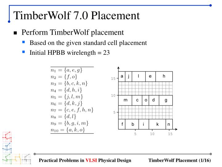
1. TimberWolf 7.0 Placement • Perform TimberWolf placement • Based on the given standard cell placement • Initial HPBB wirelength = 23 Practical Problems in VLSI Physical Design

2. First Swap • Swap node b and e • We shift node h: on the shorter side of the receiving row • Node b included in nets {n3, n9}, and e in {n1, n7} Practical Problems in VLSI Physical Design

3. Computing ΔW • ΔW = wirelength change from swap Practical Problems in VLSI Physical Design

4. Estimating ΔWs • ΔWs = wirelength change from shifting • h is shifted and included in n4 = {d,h,i} and n7 ={c,e,f,h,n} • h is on the right boundary of n4: gradient(h)++ • h is not on any boundary of n7: no further change on gradient(h) Practical Problems in VLSI Physical Design

5. Estimating ΔWs (cont) Practical Problems in VLSI Physical Design

6. Accuracy of ΔWs Estimation • How accurate is ΔWs estimation? • Node h is included in n4 = {d,h,i} and n7 ={c,e,f,h,n} • Real change is also 1: accurate estimation Practical Problems in VLSI Physical Design

7. Estimation Model B • Based on piecewise linear graph • Shifting h causes the wirelength of n4 to increase by 1 (19 to 20) and no change on n7 (stay at 28) Practical Problems in VLSI Physical Design

8. Second Swap • Swap node m and o • We shift node d and g: on the shorter side of the receiving row • Node m included in nets {n5, n9}, and o in {n2, n10} Practical Problems in VLSI Physical Design

9. Computing ΔW • ΔW = wirelength change from swap Practical Problems in VLSI Physical Design

10. Estimating ΔWs • Cell d and g are shifted • d is included in n4 = {d,h,i}, n6 ={d,k,j}, and n8 ={d,l} • d is on the right boundary of n6 and n8 • So, gradient(d) = 2 Practical Problems in VLSI Physical Design

11. Estimating ΔWs (cont) • Cell d and g are shifted • g is included in n1 = {a,e,g}, and n9 ={b,g,i,m} • g is on the right boundary of n1 and n9 • So, gradient(g) = 2 Practical Problems in VLSI Physical Design

12. Estimating ΔWs (cont) Practical Problems in VLSI Physical Design

13. Third Swap • Swap node k and m • We shift node c: on the shorter side of the receiving row • Node k included in nets {n3, n6 , n10}, and m in {n5, n9} Practical Problems in VLSI Physical Design

14. Computing ΔW • ΔW = wirelength change from swap Practical Problems in VLSI Physical Design

15. Estimating ΔWs • Cell c is shifted • c is included in n3 = {b,c,k,n} and n7 ={c,e,f,h,n} • c is on the left boundary of n3 • So, gradient(c) = −1 Practical Problems in VLSI Physical Design

16. Estimating ΔWs (cont) Practical Problems in VLSI Physical Design