Download
1 / 28
280 likes | 352 Views
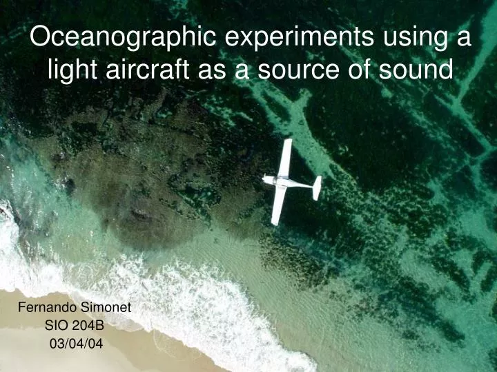
Oceanographic experiments using a light aircraft as a source of sound. Fernando Simonet SIO 204B 03/04/04. Overview. Motivation for measurements of acoustic properties of sediments Experimental setup Introduction of the aircraft as a low-frequency sound source Experiments off La Jolla, CA

E N D
Oceanographic experiments using a light aircraft as a source of sound Fernando Simonet SIO 204B 03/04/04
Overview • Motivation for measurements of acoustic properties of sediments • Experimental setup • Introduction of the aircraft as a low-frequency sound source • Experiments off La Jolla, CA • Beamforming results • Conclusions
Experimental setup • 11-element VLA • Sediment phones • Compressional • Shear • 16 channel portable DAQ • R/V Diamond Star • R/V MPL Boston Whaler
11-element VLA • Quadrupled nested with 5 elements per nesting • 250, 500, 1000 and 2000 Hz • ITC hydrophones • Sea state zero with -157 dB re 1v/uPa • 30 to 75000 Hz Omnidirectional response • Built-in low noise 20 dB pre-amps • Built-in compass and tilt sensor • Hand deployable
Sediment phones • Reson hydrophones • Compressional wave • Buried ~1m deep • Sea state zero with -186 dB re 1v/uPa sensitivity • 15 Hz to 480 kHz Omnidirectional response • Built-in 26 dB low noise pre-amp • NRL Shear sensor (bender) • Shear wave • Buried ~1m deep • -160 dB re 1uPa/V • 20 to 20000 Hz flat response • Built-in low noise pre-amps
DAQ System • Compact form factor PC (PXI) • Runs Win2K and LabVIEW • 12 VDC Battery powered • 16 simultaneously sampled channels • Max sample rate of 102400 Hz • Very high dynamic range (24 bit) • On board LPF
4 seater, single engine, light aircraft Lycomming 180 hp engine 8 m long and 12 m wing span 217 km/h (120 kts) cruise speed 3 blade wooden propeller 1100 km range 5.46 m/s (1070 ft/min) rate of climb 105 dollars/hour R/V Diamond Star
R/V MPL Boston Whaler • 2 seater, single engine, light motor vessel • Mercury 75 hp engine • 5 m long and 2 m beam • 45 km/h (25 kts) cruise speed • 4 blade metal propeller • 90 km range • 15 dollars/hour
Overview • Motivation for low-frequency measurements of acoustic properties of sediments • Experimental setup • Introduction of the aircraft as a low-frequency sound source • Experiments off La Jolla, CA • Beamforming results • Conclusions
Aircraft as a source of low-frequency sound • Propeller noise gives tonal set with usable frequency range from 80-1000 Hz. • Inexpensive and highly mobile source of low frequency sound. • Motion of aircraft gives characteristic Doppler shift.
Using Doppler-shifted frequency to identify individual rays • Each ray is launched with a different frequency • The ray retains that frequency along its entire path fDmax fD f0
Sound Speed Using Doppler Shift • Use direct ray • Received frequency is a function of local sound speed • Higher local sound speeds result in lower Doppler shifts
Measurement of sediment attenuation • Use direct ray • Compare received level at different times – i.e. different pathlengths in the sediment • Received level is a function of • Attenuation along ray path • Ray spreading
Water column measurements • Estimate the Reflection Coefficient as a function of grazing angle by comparing direct and reflected ray • Ray spreading • Attenuation along ray path • Critical angle region gives c,. • Near-normal incidence gives ρ. cs ρ
Overview • Motivation for low-frequency measurements of acoustic properties of sediments • Experimental setup • Introduction of the aircraft as a low-frequency sound source • Experiments off La Jolla, CA • Beamforming results • Conclusions
Experiments • Series of 5 experiments were conducted off the coast of La Jolla to test the feasibility of an aircraft as a source for underwater acoustics experiments • Needed to determine the potential for received signals in the water and the sediment
Data from July 2, 2002 • Temperature and pressure profile (Sea-Bird T&P Profiler SBE 39) • Microphone 1 m above the air/sea interface • 7 Hydrophones spanning much of the 15 m water column • Buried hydrophone
Some Preliminary Resultsfor Sediment Sound Speeds • Used minimization technique with a cost function that maximized power along Doppler shift curve • Started with microphone data – get v, h, ca, t0 and f0 • Proceeded to water column and sediment to get cw,cs
Application of Minimization Technique to Air Data • Microphone data • Predicts average sound speed in air (342.3 m/s) consistent with temperature conditions (343.5m/s) • Showed a flight direction bias of about 5 m/s, consistent with a wind effect (verified in GPS data) • Average aircraft velocity (54.5 m/s) in good agreement with average velocity from GPS data (54.8 m/s)
Water and Sediment Data • Water data • Acoustic data • ĉ = 1529.5 m/s • = 23.4 m/s • Sea-Bird data • ĉ = 1512.4 m/s • Sediment data • Acoustic data • ĉ = 1649 m/s • = 23.6 m/s
Overview • Motivation for low-frequency measurements of acoustic properties of sediments • Experimental setup • Introduction of the aircraft as a low-frequency sound source • Experiments off La Jolla, CA • Beamforming results • Conclusions
Beamforming on data • Diamond data (top) from 10/20/03, Cessna data (center) from 10/15/03 and simulated data (bottom) • Using all-in-one beamforming and looking at the high frequency bins (narrow main lobe) • Clear CPA offsets • 5 m on Diamond • 23 m on Cessna • Aircraft tracking • Reflection coefficient
Some concerns… • Studying a 2-D problem but in reality it’s 3-D • Surface roughness • Stable source?
Conclusions • Sound from an aircraft can be detected at reasonable levels in the water column and in the sediment • Measurement of the Doppler shift gives air/water/sediment sound speed estimates • Measurements of attenuation and dispersion may also be possible • Ability to do sediment and watersound speed measurements simultaneously • Aircraft tracking and reflection coefficient through beam forming • Using a model to better understand environment
Acknowledgments Eric Giddens Michael Buckingham ONR ARCS Foundation Thomas Hahn