Download

1 / 19
200 likes | 546 Views
Acceptance Sampling. and the evils thereof……. Rationale: (I don’t buy the argument, but…….).

E N D
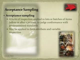
Acceptance Sampling and the evils thereof…….
Rationale: (I don’t buy the argument, but…….) In situations where Producers and Consumers are willing to put up with shipments of goods which contain defects, the issue then becomes how to keep Lots (shipments) with an “excessive” number of defects from being accepted. In order to keep Appraisal costs down, sampling schemes are devised to sample items from the Lot and then to accept or reject the Lot based upon the number of defective items found in the sample.
Notation • N= number of items in the Lot. • n= number of items in the random sample of items taken from the Lot. • D= number (unknown) of items in the Lot which are defective. • r= number of defective items in the random sample of size n. • c= acceptance number; if r is less than or equal to c then the Lot is deemed to be of Acceptable Quality, otherwise the Lot is rejected.
Acceptance Sampling Plan An Acceptance Sampling Plan is defined by: • N= Lot size • n=sample size • c=acceptance number
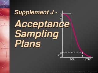
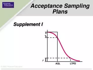
Acceptance Probability and Risks Assuming: We can evaluate a sampling plan with its corresponding Operating Characteristic Curve, a.k.a. OC curve.
Calculating probabilities for the OC curve The probabilities used in calculating values for the OC curve are calculated using the Hypergeometric Distribution. Given that then the probability that the number of defectives in the sample of size n is equal to r is given by
Acceptable Quality Level-AQL If the Lot has a proportion of defectives lower than the AQL, i.e. then the Lot is deemed to be of Acceptable Quality Level by Producer and Consumer.
OC curve and Producer and Consumer Risk The Probability that we accept a Lot is for a given proportion of defectives which is calculated using the Hypergeometric Distribution as given.
Risks and the AQL • If the proportion defective is less than or equal to the AQL, then the Producer runs the risk of having the Lot rejected which is: • If the proportion of defectives is greater than the AQL, then the Consumer runs the risk of accepting a Lot of unacceptable quality which is:
Suppose AQL=5% If the AQL=5%, we might think that the sample proportion which does not exceed 5% would indicate that the Lot is acceptable. Let us suppose our Lot size=1,000. If we plot we can see how well various plans work.
They can work if……… • If the Lots are either really good (very few defects), or really bad (many defectives). • The samples are “representative”, i.e. close to the true proportion of defectives. “Representative” is not the same as “random”. • Random samples are chosen in such a way that every possible subset is equally likely. • Only large samples are likely to be representative.
Producer and Consumer Risks • If n=20, the producer’s risk at the AQL is around 30%, i.e. a Lot of acceptable quality may be rejected. • At just over 5% defective, the Consumer’s risk is about 70%. • The plans work better as n increases.
When does random sampling start to work well? • As n increases, we would expect the Producer’s and Consumer’s risk to both decrease. • How much do we have to sample to reach an “acceptable level” of risk for both of them.
More sampling clearly does work • If we compare n=20 to n=100, there is a substantial improvement. • If we compare n=100 to n=240, there is still an improvement, but the amount of improvement is not as great, i.e. there is a diminishing return.
Largest sampling plans comparison • The largest sampling plan, n=500 has the best performance in terms of risk, but it is not much better than n=100 or n=240. • The only way to get no risk is to sample everything, or….. • Invest in Prevention, then only use sampling to monitor the improved processes.