Download
1 / 35
350 likes | 456 Views
Evaluations of Global Geophysical Fluid Models Based on Broad-band Geodetic Excitations. Wei Chen * Wuhan University, Wuhan, China Jim Ray National Oceanic and Atmospheric Administration, Silver Spring, Maryland, USA April 20, 2012.

E N D
Evaluations of Global Geophysical Fluid Models Based on Broad-band Geodetic Excitations Wei Chen* Wuhan University, Wuhan, China Jim Ray National Oceanic and Atmospheric Administration, Silver Spring, Maryland, USA April 20, 2012 * Now at Shanghai Astronomy Observatory, CAS, Shanghai, China Email: weichen.geo@gmail.com
Outline • Broad-band Geodetic Excitations • Why are the broad-band geodetic excitations needed? • How to obtain them and are the methods reliable? • Global Geophysical Fluid Models • Inter-comparisons among geophysical excitations derived from these models • Evaluations of the geophysical excitations using geodetic excitations • Role of Greenland ice in global hydrological excitation • Constructing combined geophysical excitations from different models • Discussions and Conclusions
Broad-band Geodetic Excitations • Why are the broad-band geodetic excitations needed? • To evaluate the geophysical excitations from seasonal to daily/subdaily time scales, and gain more knowledge on geophysical fluids • To quantify the IB/NonIB effect in the atmosphere-ocean interactions • Methods to derive the geodetic excitations • Wison85 filter (Wilson, 1985, Geophs J RAS) • Kalman filter (Brzezinski, 1992, Manu Geod) • Two-stage filter (Wilson & Chen, 1996, J Geod) • Gain adjustment (Wilson & Chen, 1996, J Geod) • Cubic spline fit (Kouba, 2006, J Geod) All the PM data used here are daily sampled or decimated to daily sampled with a lowpass filter Methods realized Method not realized by us
Theoretical Aspects Wilson85 filter has perfect phase but over-estimated gain w.r.t. the theoretical formula
Theoretical Aspects • Variant of the Wilson85 filter (Wilson85v) Wilson85 Linear interpolation Smoothing! Wilson85v
Comparisons of Different Methods • Wilson85 vs Wilson85v (The IG1/IGS PM data are used) Wilson85v filter would not be recommended!!! Artificial power loss caused by Wilson85v filter Wilson85v filter is adopted by the IERS-EOC webpage tool The tool is only suitable for seasonal excitations!
Comparisons of Different Methods • Wilson85 vs Gain adjustment vs Cubic spline fit Gain adjustment might be better!!! High-frequency correction caused by Gain adjustment High-frequency power loss caused by Cubic spline fit Wilson85v smoothing effect >> Gain adjustment correction
Comparisons of Different Methods • Gain adjustment vs Two-stage filter Gain adjustment is almost equivalent to Two-stage filter
Comparisons of Different Methods • Gain adjustment vs Two-stage filter Hereafter we use Gain adjustment to derive the geodetic excitations from various PM data!!! The PSD difference between them are quite small Gain adjustment and Two-stage filter are recommended
Geodetic Excitations • Geodetic excitations derived from the IERS 08 C04, IG1/IGS and SPACE2010 polar motion data Since 1997, the differences among various PM data reduced significantly!!! Since 1997, the IGS data have dominant contributions to the IERS and SPACE data Time-domain comparisons
Geodetic Excitations • Geodetic excitations derived from the IERS 08 C04, IG1/IGS and SPACE2010 polar motion data Differences lie in high-frequency bands!!! PM data: 1994 - 2010 High-frequency components of C04 are quite suspect before 2007 PM data: 1997 - 2010 Frequency-domain comparisons
Geodetic Excitations • Geodetic excitations derived from the IERS 08 C04, IG1/IGS and SPACE2010 polar motion data These data agree with each other quite well at low frequency bands Frequency-domain comparisons
Global Geophysical Fluid Models • To study the global geodynamics, various atmospheric, oceanic and hydrological models are established • Different versions of the global geophysical models • NCEP/NCAR (National Centers for Environmental Prediction/National Center for Atmospheric Research) reanalyses: AAM, HAM • ECMWF (European Centre for Medium-Range Weather Forecasts) reanalyses: AAM, OAM, HAM • JMA (Japan Meteorological Agency) products:AAM • UKMO (United Kingdom Meteorological Office) products:AAM • ECCO (Estimating the Circulation and Climate of the Ocean) Assimilation products: OAM • GLDAS (Global Land Data Assimilation System) products: HAM JMA and UKMO AAMs are not used since there are not OAMs consistent with them
Model Evaluations I: Daily data • Data used • IERS EOP 08 C04 (1997 ~ 2008) • NCEP reanalysis AAM + ECCO kf080 OAM + NCEP reanalysis HAM (1997 ~ 2008) • ECMWF ERA40 (1997 ~ 2001) plus ECMWF operational (2002 ~ 2008) AAM + OAM + HAM • Formula of Eubanks (1993) is used to derive the effective geophysical excitations • Inverted barometer (IB) assumption is adopted to combine AE and OE
Time Series Comparisons (1d) AE matter OE matter Good agreements for AE! ECMWF OE has stronger signals than ECCO one OE motion AE motion
Time Series Comparisons (1d) • Even for the same model GLDAS, the HEs are quite different!!! • GLDAS(Yan).HE (cyan line) is provided by Dr. Haoming Yan • GLDAS.HE (red line) is our estimate (Monthly data tws_gldas_noah_1m_7901_1010.dat is used) Poor agreements for HE!
Excess Polar Motion Excitations (1d) Residuals contain strong semi-annual signals
Spectrum Comparisons (1d) Possible long-period bias in ECMWF HE Here long-period bias means long-period error
Spectrum Comparisons (1d) Possible long-period bias in GLDAS HE Long-period errors in GLDAS surface loading was also found by a comparison with the GPS observations (Ray & van Dam, 2011, private communication) Annual signals of NCEP HE are too strong
Coherence Comparisons Adding HE reduces the coherence with Obs Coherences between GE, AEs, (AE + OE)s and (AE+OE+HE)s
Coherence Comparisons with IGS and SPACE Only AEs and OEs are used while HEs are excluded
Effect of debias Here debias means removing the long-period error Debias removes the low-frequency discrepancies
Role of Greenland TWS • On the GLDAS-based HE • Yan’s estimate is different from ours • H. Yan (2010, private communication): set the TWS to 500 mm equivalent water height in Greenland • J. L. Chen & C. Wilson (2005): without details • This study: TWS in Greenland not changed • Is the difference due to different treatments of the TWS in Greenland • (or) Is the Greenland water storage important in the estimate of the hydrological excitation?
Greenland TWS • Taking the GLDAS model as an example GLDAS grid data (1 degree by 1 degree, in meter) for Jan. 1979 The maximal value of the equivalent water height can reach a few meters! Here we impose a 1-m limit to show the details of TWS in most areas.
HEs estimated from GLDAS Model With or without Greenland TWS seems not important
HEs estimated from GLDAS Model Effects of Greenland TWS on hydrological excitation are quite small! The difference is ~0.5 mas at most
Model Evaluations II: 6-h data • Data used(2004 ~ 2010) • IGS EOP: ig1+igs+igu.erp (6-hour data; a combination of the IGS/IG1 and the IGU polar motion data) • NCEP reanalysis AAM (6h) + ECCO kf080 OAM (#) + NCEP reanalysis HAM (#) • ECMWF operational AAM (6h) + OAM (6h) + HAM (#) • ERAinterim AAM (6h) + OAM (6h) + HAM (#) • COMB: combined AAM (6h) + OAM (6h) + HAM (6h) (#) originally daily, linearly interpreted to 6-hour data “COMB” refers to the combination of the three different sets of geophysical fluid models. We use a “least difference method” to combine these models, that is, we choose the data points which are the closest to the observations from the aspects of magnitude and phase (see Chen, 2011)
Time Series Comparisons (6h) AE matter OE matter Values of COMB OE lie between those of ECMWF OE and ECCO OE AE motion OE motion
Time Series Comparisons (6h) The residual for COMB is a little smaller!
Coherence Comparisons (6h) COMB is the most coherent with the Obs!
Spectrum Comparisons (6h) Compared with GE: NCEP/ECCO: signals too weak ECMWF/ERAinterim: signals too strong! The PSD for COMB agrees best with the Obs!
Discussions and Conclusions • IERS C04 EOP might be problematic before 1997 • Widely adopted Wilson85 filter is only suitable for seasonal excitation studies • To derive broad-band geodetic excitations, two-stage filter and gain adjustment are recommended • Biases actually exist in the ECMWF and GLDAS hydrological models, While NCEP model over-estimates the annual variation in the TWS • Effect of the Greenland is not significant (no more than 0.5 mas) • Reliability atmospheric model > oceanic model > hydrological model • Combined geophysical fluid models might be better
Acknowledgement • Richard Gross provided us the JPL SPACE data (v2010) • Haoming Yan provided us his estimate of the GLDAS HE
References • Brzeziński, A. (1992) Polar motion excitation by variations of the effective angular momentum function: considerations concerning deconvolution problem, Manuscr. Geod., 17: 3–20. • Chen, J.L., Wilson, C.R. (2005) Hydrological excitations of polar motion, 1993-2002. Geophys. J. Int., 160: 833–839. • Chen, W. (2011) Rotation of the triaxially-stratified Earth with frequency-dependent responses, Ph.D. Thesis, Wuhan University, Wuhan, China. • Eubanks, T.M., 1993. Variations in the orientation of the Earth. In Contributions of Space Geodesy to Geodynamics: Earth Dynamics, Geodyn. Ser., vol. 24, edited by D. E. Smith and D. L. Turcotte, pp. 1–54, AGU, Washington, D. C. • Kouba, J. (2005) Comparison of polar motion with oceanic and atmospheric angular momentum time series for 2-day to Chandler periods, J. Geod., 79: 33–42. • Ray, J. (2009) Status and prospects for IGS polar motion measurements, http://acc.igs.org/studies.html • Wilson, C.R. (1985) Discrete polar motion equations. Geophys. J. R. Astron. Soc. 80, 551–554. • Wilson CR, Chen JL (1996) Discrete polar motion equations for high frequencies. J. Geod. 70, 581–585.
Thanks for your attention!Presented at the GGFC workshop, Vienna, Austria, April 20, 2012