Download
1 / 19
190 likes | 336 Views
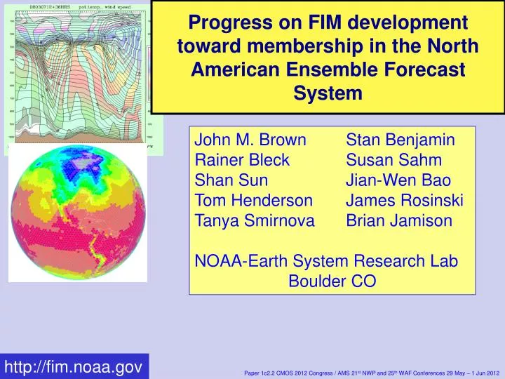
Progress on FIM development toward membership in the North American Ensemble Forecast System. John M. Brown Stan Benjamin Rainer Bleck Susan Sahm Shan Sun Jian-Wen Bao Tom Henderson James Rosinski Tanya Smirnova Brian Jamison NOAA-Earth System Research Lab Boulder CO.

E N D
Progress on FIM development toward membership in the North American Ensemble Forecast System John M. Brown Stan Benjamin Rainer Bleck Susan Sahm Shan Sun Jian-Wen Bao Tom Henderson James Rosinski Tanya Smirnova Brian Jamison NOAA-Earth System Research Lab Boulder CO http://fim.noaa.gov Paper 1c2.2 CMOS 2012 Congress / AMS 21st NWP and 25th WAF Conferences 29 May – 1 Jun 2012
X-section location Flow-following- finite-volume Icosahedral Model FIM Temp at lowest level Original concept and early work on FIM was by Sandy MacDonald and Jin Lee, ESRL
FIM numerical model • Horizontal grid • Icosahedral, Arakawa A grid – testing 60km/30km/15km • Vertical grid • Staggered Lorenz grid, ptop = 0.5 hPa, θtop ~2200K • Generalized vertical coordinate • Hybrid θ-σ option (64L, 38L, 21L options currently) • Hybrid σ-p option (64L, identical to GFS) • Numerics • Adams-Bashforth 3rd order time differencing • Flux-corrected transport • Physics • GFS physics suite (May 2011 version, work underway on Q3FY12 version) • Coupled model extensions • Chem – WRF-chem/GOCART (Georg Grell) • Ocean – icosahedral HYCOM (Shan Sun 1030 Friday)
Novel features of FIM: • Finite-volume Integrations on Local Coordinate • Efficient Indirect Addressing Scheme on Irregular Grid • MacDonald, Middlecoff, Henderson, and Lee (2010, IJHPC) : • A General Method for Modeling on Irregular Grids. • FIM: Hybrid σ-θ Coordinate • - Bleck, Benjamin, Lee and MacDonald (2010, MWR): On the Use of an Arbitrary Lagrangian-Eulerian Vertical Coordinate in Global • Atmospheric Modeling. • Conservative and Monotonic 3rd-ord Adams-Bashforth w/ FCT Scheme • - Lee, Bleck, and MacDonald (2010, JCP): A Multistep Flux-Corrected Transport Scheme • Grid Optimization for Efficiency and Accuracy • - Wang and Lee (2011, SIAM): Geometric Properties of Icosahedral-Hexagonal Grid • on Sphere. Lee and MacDonald (MWR, 2009): A Finite-Volume Icosahedral Shallow Water Model on Local Coordinate. NOAA Earth System Research Laboratory - Boulder, Colorado
Sadourny, Arakawa, Mintz, MWR (1968) Construction of an icosahedral grid high granularity possible with icosahedral model Bisection: N=(2**m)*10 + 2 “m” is any integer ratio between arc A-B (~8000 km) and target resolution. e.g., for dx~20 km, then m=8000/20=400 N=(400**2)*10+2~1.6 million points. FIM – Ning Wang (ESRL) Can use arbitrary sequence of bisections and trisections
The 2-D operator applied to the straight lines, rather than the 3-D operator along the curved lines, e.g., Stokes’ theorem: Local stereographic projection for each icosahedral grid volume for local geometry
FIM design – vertical coordinate • Hybrid (sigma/ isentropic) vertical coordinate • Improved transport by reducing numerical dispersion from vertical cross-coordinate transport, improved stratospheric/tropospheric exchange. • Used in NCEP Rapid Update Cycle (RUC) model • Used in HYCOM ocean model Installed as generalized “s” vertical coordinate - can be replaced with GFS sigma-p or other coordinates.
Staggering of variables in layer or stacked shallow-water models: Used in FIM
FIM vertical coord hybrid σ-θ-σ option • 2 σ layers at top • θv reference values for all levels • σ layers at surface set at max=15 hPa θ-σ
Continuity equation in generalized (“s”) coordinates (~zero in fixedgrids) (~zero in material coord.) (known)
Initial Physics in FIM GFS physics • Immediate goal for FIM is contributing dynamical-core diversity to NCEP Global Ensemble Forecast System • Use of current GFS physics (Fanglin Yang’s talk 1B1.2, previous session)allows evaluation of differences between GFS and FIM dynamical cores. Application of GFS physics to FIM • No changes needed to physics for hybrid θ-σ application with one exception: mod to avoid negative mass flux in deep/shallow cu, no change to GFS performance • Applied every 180s (multiple explicit time-steps in FIM) Current retrospective experiments with Grell-3D replacing GFS deep/shallow cumulus
Key Recent FIM Changes • April 2011 • Fix to FCT numerics (error in high-order fluxes) • Nov 2011 • Upgrade from GFS 2010 physics to May-2011 GFS physics • Addition of icosahedral momentum diffusion (upgraded to 4th order April 2012) • Currently working on upgrade to May 2012 GFS physics (major code upgrade; only minor changes to actual physics)
Track Error -2011 Atlantic/e.Pacific Tropical Cyclones • GFS oper • FIM30km real-time (EnKF IC) • FIM30km retro (hybrid IC) • FIM15km retro (hybrid IC)
500hPa Height Anomaly Correlation 20o – 80o North Latitude, 00UTC only N = 88 Avg s.d. FIM 87.72 5.05 GFS 87.51 5.12
72h forecasts vs. raobs N. Hemisphere 20-80N FIM vs. GFS (FIM lower rms errors for V, T, RH at all levels, similar results at 24h,48h) FIM better FIM better FIM better GFS better GFS better GFS better
Summary • Overall FIM performance roughly equal to GFS using GFS initial conditions • FIM forecasts often similar to GFS at 5 days, but sometimes quite different. • FIM and GFS “dropouts” often don’t occur at same initial time • Significant improvement in FIM from 2011 to 2012 (hurricane track errors reduced by 20%) • Best FIM performance for wind, RH, temp • Less so for heights
NOAA/ESRL/GSD Assimilation and Modeling Branchpresentations on regional and global NWP Tue 14:15 Global model (FIM) development (John Brown) Tue 15:15 Boundary-layer wind simulation in low-level jets (Joe Olson) Tue 17:30 Gridpoint Statistical Interpolation for Rapid Refresh (Ming Hu) Wed 16:30 Storm-scale radar-data assimilation (David Dowell) Wed 17:00 High-Resolution Rapid Refresh climatology (Eric James) Wed 17:15 GSI cloud analysis and rawinsonde DA (Patrick Hofmann) Thu 10:45 Rapid Refresh implementation at NCEP (John Brown) Thu 11:00 High-Resolution Rapid Refresh overview (Curtis Alexander) Thu 17:30 NWP guidance for a high-impact snowstorm (Ed Szoke) Fri 10:30 Spatial discretization for global models (Shan Sun) Fri 17:00 Snow and ice enhancements for RUC LSM (Tanya Smirnova)
Brief summary of GFS Physics Radiation: Rapid Radiative Transfer Model for both long and short wave Surface processes: Noah LSM over land surface fluxes using variable drag coefficient over sea simple sea-ice model PBL: Han and Pan (NCEP Office Note #464) based on Troen and Mahrt, extra vertical mixing at Sc cloud top if entrainment instability criterion met Shallow and deep convection: Han and Pan (NCEP Office Note #464) mass flux scheme Explicit condensate allowed, Zhao and Carr (19xx, MWR) (including simple ice processes)