Download

1 / 50
520 likes | 1.05k Views
Bistability in Biochemical Signaling Models. Eric Sobie Pharmacology and Systems Therapeutics Mount Sinai School of Medicine eric.sobie@mssm.edu. 1. Outline: Part 1. Some biological background Biological importance of bistability Qualitative requirements of bistability

E N D
Bistability in Biochemical Signaling Models Eric Sobie Pharmacology and Systems Therapeutics Mount Sinai School of Medicine eric.sobie@mssm.edu 1
Outline: Part 1 Some biological background Biological importance of bistability Qualitative requirements of bistability How to predict if bistability will be present? Rate-balance plots Dynamical systems analyses Examples of bistability An artificial genetic "toggle switch" MAP-kinase pathway in oocyte maturation MAP-kinase pathway in mammalian cells 2
What is bistability? A situation in which two possible steady-states are both stable. In general, these correspond to a "low activity" state and a "high activity" state. Ferrell & Machleder (1998) Science280:895-898. Between stable steady-states, an unstable steady state will be present. 3
Biology: generally monostable and analog Epinephrine increased cardiac output Increased blood glucose insulin production Enzyme conversion of substrate to product response Cardiac output [insulin] d[Product]/dt [epinephrine] [blood glucose] [E] stimulus Response depends directly on level of stimulus When stimulus is removed, response returns to prior level 4
Fertilization Cell division Differentiation Action potentials Apoptosis T-cell activation When is analog not good enough? For these processes, a graded response is inadequate These phenomena also require persistence 5
At the biochemical level, how does bistability arise? Mutual activation Mutual inhibition Ferrell (2002) Curr. Op. Cell Biol.14:140–148. These types of circuits CAN produce bistability, but they do NOT guarantee bistability This is why we need quantitative analyses 6
[G] [ATP] Bistability in terms of dynamical behavior Previously we encountered stable and unstable fixed points and limit cycles Km = 13 Km = 20 The fixed point is “unstable.” The oscillation is a “stable limit cycle.” The fixed point is “stable.” 7
[LacY] [LacY] Time Time Bistability in terms of dynamical behavior A monostable system A bistable system Multiple steady states are possible Initial conditions determine which steady state is reached 8
Quantitative analyses of bistability 1) A simple "Michaelian" system A* = phosphorylated A Total amount of [A] is constant: We want to solve for [A*] in the steady-state or 9
Rate balance plots Instead of solving equations, find solution graphically Backward Rate Forward Rate At steady-state, FR = BR Rate Backward Forward 0 0.5 1 [A*]/[A]TOTAL analysis based on Ferrell & Xiong (2001) Chaos 11:227-236. 10
Rate balance plots Very closely related to phase line plots At steady-state, FR – BR = 0 4 2 [A*]/[A]TOTAL d[A*]/dt 0 0.5 1 -2 -4 -6 Intuitively, then, this fixed point is stable 11
Stability analysis of ODE systems A one-dimensional example Isolated cardiac myocyte 10 8 Stable fixed point 6 Unstable fixed point 4 dV/dt (mVms) 2 0 -2 -4 -100 -90 -80 -70 -60 V (mV) Change to < -85 positive dV/dt Change to ~-70 negative dV/dt Change to >~-58 positive dV/dt Beginning with a myocyte at rest (-85 mV), simulate instantaneous changes in voltage, calculate Iion 12
0 0.5 1 Rate balance plots Now, assume that forward rate is function of stimulus: Plot rate balance for different values of stimulus [S] Big [S] Rate Backward Small [S] [A*]/[A]TOTAL 13 13
1 0.5 0 0 10 20 30 Rate balance plots This analysis can be used to plot [S] versus [A*]/[A]TOTAL [A*]/[A]TOTAL Rate 0 0.5 1 [S] [A*]/[A]TOTAL 14
Rate balance plots 2) Michaelian system with linear feedback kf determines strength of feedback Weak feedback Strong feedback Forward Rate Rate Backward 0 1 0 1 [A*]/[A]TOTAL [A*]/[A]TOTAL The right plot "looks" bistable. Is it? 15
How can the "off" state be made stable? Strong feedback Forward Rate Backward 0 0.5 1 [A*]/[A]TOTAL Two ways this can be modified to be truly bistable 1) Nonlinear ("ultrasensitive") feedback 2) Partial saturation of the back reaction 16
Rate balance plots 3) Michaelian system with ultrasensitive feedback Rate 0 0.5 1 [A*]/[A]TOTAL Now we have a bona fide bistable system 17
Rate balance plots 3) Michaelian system with ultrasensitive feedback Effects of changes in hill exponent n n = 8 n = 2 Rate n=4 0 0.5 1 [A*]/[A]TOTAL 18
Rate balance plots 4) Linear feedback plus saturating back reaction Rate 0 0.5 1 [A*]/[A]TOTAL 19
Rate balance plots How can the cell change states? Vary the amount of stimulus [S] Last couple of slides assumed [S]=0 0.9 0.6 [A*]/[A]TOTAL Rate 0.3 0 [S] 0 0.5 1 0 0.5 1 [A*]/[A]TOTAL Where the system switches between 3 and 1 steady states is a bifurcation 20
Switching can be reversible or irreversible Ferrell (2002) Curr. Op. Cell Biol. 14:140–148. In either case, bistability implies hysteresis 21
0.7 0.6 0.5 0.4 0.3 0.2 0.1 0 0 2 4 6 8 10 12 14 16 18 20 Analysis of two variable systems Dynamical systems theory and nullclines 1) Generic example of mutual activation Tyson (2003) Curr. Op. Cell Biol.15:221-231 low initial [R] Steady state [R] high initial [R] [S] 22
35 30 25 20 15 10 5 0 0 2 4 6 8 10 12 14 Analysis of two variable systems 2) Generic example of mutual repression Tyson (2003) Curr. Op. Cell Biol.15:221-231 low initial [R] Steady state [R] high initial [R] [S] 23
16 12 [Glucose] 8 4 0 0 4 8 12 [ATP] Analysis of two variable systems In 2D phase plane, direction determined by: Plot direction vectors in the Bier model d[G]/dt = 0 Consider [ATP] big; [G] big: d[ATP]/dt = 0 Each time you cross a nullcline, one of these changes direction! The system will proceed in a clockwise direction (stability is unclear) Nullclines divide the phase space into discrete regions 24
25 20 15 10 5 0 0 0.5 1 Analysis of two variable systems 2) Generic example of mutual repression What do the nullclines look like? R nullcline d[E]/dt = 0 E nullcline d[R]/dt = 0 [R] [S]=10 [S]=6 [S]=2 [E] Transition from 3 intersections to 1 intersection = bifurcation 25
Examples of bistable systems An artificial "toggle switch" Gardner, Cantor, & Collins (2000) Nature339-342 26
Examples of bistable systems MAPK cascade in oocyte maturation Ferrell & Machleder (1998) Science 280:895-898 27
Examples of bistable systems MAPK cascade in mammalian cells Bhalla & Iyengar (1999) Science 283:381-387 28
Part 2 29
Outline: Part 2 Review of important ideas from Tuesday Concepts underlying rate balance plots How these plots were generated in MATLAB Assessing stability in two-dimensional systems The mathematically rigorous method A qualitative graphical method The E. coli lac operon Basic biology A simple model Homework assignment 30
At the biochemical level, how does bistability arise? Mutual activation Mutual inhibition Ferrell (2002) Curr. Op. Cell Biol.14:140–148. These types of circuits CAN produce bistability, but they do NOT guarantee bistability This is why we need quantitative analyses 31
0 0.5 1 Rate balance plots Now, assume that forward rate is function of stimulus: Plot rate balance for different values of stimulus [S] Big [S] Rate Backward Small [S] [A*]/[A]TOTAL 32
Rate balance plots 3) Michaelian system with ultrasensitive feedback Rate 0 0.5 1 [A*]/[A]TOTAL Now we have a bona fide bistable system 33
Rate balance plots How can the cell change states? Vary the amount of stimulus [S] Last couple of slides assumed [S]=0 0.9 0.6 [A*]/[A]TOTAL Rate 0.3 0 [S] 0 0.5 1 0 0.5 1 [A*]/[A]TOTAL Where the system switches between 3 and 1 steady states is a bifurcation 34
Switching can be reversible or irreversible Ferrell (2002) Curr. Op. Cell Biol. 14:140–148. In either case, bistability implies hysteresis Why is hysteresis beneficial? 35
35 30 25 20 15 10 5 0 0 2 4 6 8 10 12 14 Analysis of two variable systems 2) Generic example of mutual repression Tyson (2003) Curr. Op. Cell Biol.15:221-231 low initial [R] Steady state [R] high initial [R] [S] 36
30 25 [S]=2 [S]=6 20 [S]=12 35 [R] 15 30 10 25 5 20 0 time 0 10 20 30 40 50 15 10 5 0 0 2 4 6 8 10 12 14 Analysis of two variable systems 2) Generic example of mutual repression Time course of [R] at different values of [S] low initial [R] high initial [R] Steady state [R] [S] Initial conditions determine which steady state is reached 37
14 12 10 8 6 4 2 0 10 20 30 40 50 Analysis of two variable systems 2) Generic example of mutual repression [R] vs. time at [S] = 6 25 20 E nullcline R nullcline 15 [R] [R]0 = 5.2; [E]0 = 0.5 [R]0 = 5.4; [E]0 = 0.3 [R] 10 5 [S]=6 0 Time 0 0.5 1 [E] 38
25 20 15 10 5 0 0 0.5 1 Analysis of two variable systems 2) Generic example of mutual repression What do the nullclines look like? R nullcline E nullcline R nullcline E nullcline [R] [S]=10 [S]=6 [S]=2 [E] How do we tell if the fixed points are stable or unstable? 39
Analysis of two variable systems A qualitative, graphical analysis of stability 25 [dE/dt,dR/dt] defines a direction of "movement" in the [E,R] plane E nullcline 20 On the E nullcline, dE/dt = 0, direction of movement is up/down R nullcline 15 On the R nullcline, dR/dt = 0, direction of movement is left/right [R] 10 The direction changes when a nullcline is crossed 5 0 [E] 0 0.5 1 With these simple rules, we can (often) determine stability 40
Graphical analysis of stability Examine equations to determine directions (Remember that R is the ordinate) We plot dR/dt on E nullcline We plot dE/dt on R nullcline 25 On the E nullcline, and above the R nullcline, dR/dt < 0 E nullcline 20 On the R nullcline, and above the E nullcline, dE/dt < 0 R nullcline 15 These considerations suggest that middle steady state is unstable, left and right steady states are stable [R] 10 5 0 [E] 41 0 0.5 1
Graphical analysis of stability Using the MATLAB "quiver" function E nullcline Near right, stable SS Near middle, unstable SS R nullcline [R] [R] [E] [E] Epos = linspace(Erange(1),Erange(2),quiverpoints) ; Rpos = linspace(Rrange(1),Rrange(2),quiverpoints) ; [Equiv,Rquiv] = meshgrid(Epos,Rpos) ; dR = k0r*(Etot-Equiv) + k1r*S - k2r*Rquiv ; dE = -k2e*Rquiv.*Equiv./(Km2e + Equiv) + k1e*(Etot - Equiv)./ ... (Km1e + Etot - Equiv) ; quiver(Equiv,Rquiv,dE,dR,1.2) 42
Stability analysis of ODE systems How can we understand stable and unstable fixed points mathematically? Compute the “Jacobian” matrix: Evaluate this at the fixed points defined by [E*], [R*] (This is where analytical computations become difficult) 43
25 20 15 [R] 10 5 [S]=6 0 [E] 0 0.5 1 Stability analysis of ODE systems Evaluate Jacobian matrix at the fixed points defined by [E*], [R*] The eigenvalues of the Jacobian (at the fixed points) determine stability The real part of either is positive: the fixed point is unstable Real parts of both are negative: the fixed point is stable eigenvalues = -21.0618 -0.0915 repression_stability.m computes these eigenvalues = -1.0282 0.3379 eigenvalues = -59.1985 -0.0983 44
Examples of bistable systems MAPK cascade in oocyte maturation Ferrell & Machleder (1998) Science 280:895-898 45
Examples of bistable systems MAPK cascade in mammalian cells Bhalla & Iyengar (1999) Science 283:381-387 46
Examples of bistable systems The lac operon in E. coli Smits et al. (2006) Nat. Rev. Micro. 4:259-271 With low nutrient levels, LacI will repress transcription of the the LacA, LacY, and LacZ genes. Lactose, allolactose, or IPTG will bind to LacI, relieve repression. LacY encodes a "permease,” which allows lactose into the cell. 47
Examples of bistable systems A minimal model of the lac operon l = intracellular lactose LacY = expression of LacY/permease β, γ, δ, σ, p, l0 = constants lext = external lactose (Note: in most models, dLacY/dt depends on [lactose]2. We have assumed a dependence on [lactose]4 to improve the nullcline plots.) 48
Homework assignment 1) Rate balance plots Linear autocatalytic feedback & saturation of back reaction Rate [A*]/[A]TOTAL Kmb [A*]/[A]TOTAL 2) Model of lac operon Nullcline analysis and dynamic simulations [LacY] [lactose] Time [lactose] 49
Slides from a lecture in the course Systems Biology—Biomedical Modeling Citation: E. A. Sobie, Bistability in biochemical signaling models. Sci. Signal.4, tr10 (2011). www.sciencesignaling.org