Download
1 / 65
660 likes | 707 Views
Waiting Lines and Queuing Theory Models. Introduction. The study of waiting lines, called queuing theory, is one of the oldest and most widely used Operations Research techniques.

E N D
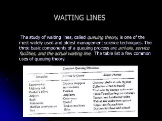
Introduction • The study of waiting lines, called queuing theory, is one of the oldest and most widely used Operations Research techniques. • Waiting lines are an everyday occurrence, affecting people shopping for groceries, buying gasoline, or making a bank deposit. • Queues, another term for waiting lines, may also take the form of machines waiting to be repaired, trucks in line to be unloaded, or airplanes lined up on a runway waiting for permission to take off. • The three basic components of a queuing process are arrivals, service facilities, and the actual waiting line. In this chapter we discuss how analytical models of waiting lines can help managers evaluate the cost and effectiveness of service systems. 14-2
Waiting Line Costs • Most waiting line problems are centered on the question of finding the ideal level of services that a firm should provide. "one of the goals of queuing analysis is finding the best level of service for an organization". • In most cases, this level of service is an option over which management has control. An extra teller, for example, can be borrowed from another chore or can be hired and trained quickly if demand warrants it. This may not always be the case, though. A plant may not be able to locate or hire skilled mechanics to repair sophisticated electronic machinery. 14-3
Waiting Line Costs\continued • When an organization does have control, its objective is usually to find a happy medium between two extremes: 1. On the one hand, a firm can retain a large staff and provide many service facilities. This may result in excellent customer service, with seldom more than one or two customers in a queue. Customers are kept happy with the quick response and appreciate the convenience. This, however, can become expensive. 2. The other extreme is to have the minimum possible number of checkout lines, gas pumps, or teller windows open. This keeps the service cost down but may result in customer dissatisfaction. "As the average length of the queue increases and poor service results, customers and goodwill may be lost." 14-4
Waiting Line Costs\continued "Managers must deal with the trade-off between the cost of providing good service and the cost of customer waiting time. The latter may be hard to quantify." • One means of evaluating a service facility is thus to look at a total expected cost, a concept illustrated in the figure (the next slide). Total expected cost is the sum of expected service costs plus expected waiting costs. • Service costs are seen to increase as a firm attempts to raise its level of service. As service improves in speed, however, the cost of time spent waiting in lines decreases. "The goal is to find the service level that minimizes total expected cost." 14-5
Queuing Costs and Service Levels Total Expected Cost Optimal Service Level Cost of Providing Service Cost of Operating Service Facility Cost of Waiting Time Service Level 14-6
Waiting Line Costs\continuedThree Rivers Shipping Company Example • Three Rivers run a huge docking facility located on the Ohio River near Pittsburgh. Approximately five ships arrive to unload their cargoes of steel and ore during every 12-hour work shift. Each hour that a ship sits idle in line waiting to be unloaded costs the firm a great deal of money, about $1,000 per hour. From experience, management estimates that if one team of stevedores is on duty to handle the unloading work, each ship will wait an average of 7 hours to be unloaded. If two teams are working, the average waiting time drops to 4 hours; for three teams, it's 3 hours; and four teams of stevedores, only 2 hours. But each additional team of stevedores is also an expensive proposition, due to union contacts. • Three rivers' superintendent would like to determine the optimal number of teams of stevedores to have on duty each shift. • The objective is to minimize total expected costs. This analysis is summarized in the next table: 14-7
Waiting Line Cost AnalysisThree Rivers Shipping Number of Stevedore Teams 1 2 3 4 Avg. number of ships arriving per shift 5 5 5 5 Average waiting time per ship 7 4 3 2 Total ship hours lost 35 20 15 10 Est. cost per hour of idle ship time $1,000 $1,000 $1,000 $1,000 Value of ships' lost time 35,000 29,000 $15,000 $10,000 Stevedore teams salary $6,000 $12,000 18,000 $24,000 Total Expected Cost $41,000 $32,000 $33,000 $34,000 14-8
Characteristics Of A Queuing System • We will study three parts of a queuing system: 1. The arrivals or inputs to the system (sometimes referred to as the calling population), 2. The queue or the waiting line itself, and 3. The service facility 14-9
1. Arrival Characteristics • The input source that generates arrivals or customers for the service system has three major characteristics. It is important to consider: • the size of the calling population, • the pattern of arrivals at the queuing system, and • the behavior of the arrivals. 14-10
1. Arrival Characteristics\continued Size of the Calling Population • Population sizes are considered to be either unlimited (essentially infinite) or limited (finite). • For practical purposes, examples of unlimited population includes cars arriving at a highway tollbooth, shoppers arriving at a supermarket, or students arriving to register for classes at large university. "Most queuing models assume such an infinite calling population". • An example of a finite population is a shop with only eight machines that break down and require service. 14-11
1. Arrival Characteristics\continued Pattern of Arrivals at the System • Customers either arrive at service facility according to some known schedule (for example, one patient every 15 minutes or one student for advising every half hour) or else they arrive randomly. • Arrivals are considered random when they are independent of one another and their occurrence cannot be predicted exactly. • Frequently in queuing problems, the number of arrivals per unit of time can be estimated by a probability distribution known as the Poisson distribution. "The Poisson probability distribution is used in many queuing models to represent arrival patterns." 14-12
Poisson Distribution for Arrival Times For X=0,1,2,3,4,…….. P(X)= probability of X arrivals X= number of arrivals per unit of time = average arrival rate e= 2.7183 14-13
Poisson Distribution for Arrival Times P(X), = 2 P(X), = 4 P(X) .35 P(X) .30 .30 .25 .25 .20 .20 .15 .15 .10 .10 .05 .05 .00 .00 0 1 2 3 4 5 6 7 8 9 10 11 0 1 2 3 4 5 6 7 8 9 10 11 X X 14-14
1. Arrival Characteristics\continued Behavior of the Arrival • Most queuing models assume that an arriving customer is a patient customer. • Patient customers are people or machines that wait in the queue until they are served and do not switch between lines. • Unfortunately, life and operations research are complicated by the fact that people have been known to balk or renege. • Balking refers to customers who refuse to join the waiting line because it is too long to suit their needs or interests. • Reneging customers are those who enter the queue but then become impatient and leave without completing their transaction. 14-15
2. Waiting Line Characteristics We will study the: • Length of the queue • Service priority/Queue discipline 14-16
2. Waiting Line Characteristics\continued Length of the queue • The length of a line can be either limited or unlimited. • A queue is limited when it cannot increase to an infinite length. This may be the case in a small restaurant that has only 10 tables and can serve no more than 50 diners an evening. • Analytic queuing models are treated in this chapter under an assumption of unlimited queue length. 14-17
2. Waiting Line Characteristics\continued Service priority/Queue discipline • Queue discipline refers to the rule by which customers in the line are to receive service. • Customers may be served according to one of the next disciplines: • first-in, first-out rule (FIFO) • priority discipline • last-come first-served (LCFS) • service in random order (SIRO) 14-18
3. Service Facility Characteristics • It is important to examine two basic properties: • the configuration of the service system • the pattern of service times 14-19
3. Service Facility Characteristics\continued Basic Queuing System Configuration • Service systems are usually classified in terms of number of channels and number of phases in service. 1. Number of channels • A single-channel system, with one server, is typified by the drive-in bank that has only one open teller. • A multi-channel system, when the bank has several tellers on duty and each customer waits in one common line for the first available teller. 14-20
3. Service Facility Characteristics\continued 2. Number of phases in service • A single-phase system, in this case the customer receives service from only one station and then exists the system. • A multiphase system, for example, if the restaurant require you to place your order at one station, pay at a second, and pick up the food at a third service stop. 14-21
Basic Queuing System Configurations Queue Service facility Single Channel, Single Phase Service Facility Queue Facility 2 Facility 1 Single Channel, Multi-Phase 14-22
Basic Queuing System Configurations Service facility 1 Queue Service facility 2 Service facility 3 Multi-Channel, Single Phase Type 2 Service Facility Type 1 Service Facility Queue Type 2 Service Facility Type 1 Service Facility Multi-Channel, Multiphase Phase 14-23
3. Service Facility Characteristics\continued The Pattern of Service Times • Service patterns are like arrival patterns in that they can be either constant or random. • If service time is constant, it takes the same amount of time to take care of each customer. This is the case in a machine-performed service operation such as an automatic car wash. • More often, service times are randomly distributed. In many cases it can be assumed that random service times are described by the negative exponentialprobability distribution. 14-24
3. Service Facility Characteristics\continued Average Service Time of 20 Minutes Probability (for Intervals of 1 Minute) Average Service Time of 1 Hour X 30 60 90 120 150 180 • The next figure illustrates that if service times follow an exponential distribution, the probability of any very long service time is low. 14-25
Identifying Models Using Kendall Notation • D.G. Kendall developed a notation that has been widely accepted for specifying the pattern of arrivals, the service time distribution, and the number of channels in a queuing model. • The basic three-symbol Kendall notation is in the form: Arrival distribution/ service time distribution/ number of service channels open Where specific letters are used to represent probability distributions. The following letters are commonly used in Kendall notation: • M= Poisson distribution for number of occurrences (or exponential times) • D= Constant (deterministic) rate • G= General distribution with mean and variance known 14-26
Identifying Models Using Kendall Notation\continued • Thus, a single channel model with Poisson arrivals and exponential service times would be represented by M/M/1 • When a second channel is added, we would have M/M/2 (An M/M/2 model has Poisson arrivals, exponential service times, and two channels) • If there are m distinct service channels in the queuing system with Poisson arrivals and exponential service, the Kendall notation would be M/M/m. 14-27
Identifying Models Using Kendall Notation\continued • A three-channel system with Poisson arrivals and constant service time would be identified as M/D/3. • A four channel system with Poisson arrivals and service times that are normally distributed would be identified as M/G/4. 14-28
Single-Channel Queuing Model With Poisson Arrivals And Exponential Service Times (M/M/1) Assumptions of the Model • The single-channel, single-phase model considered here is one of the most widely used and simplest queuing models. It involves assuming that seven conditions exist: • Arrivals are served on a FIFO basis. • Every arrival waits to be served regardless of the length of the line; that is, there is, no balking or reneging. • Arrivals are independent of preceding arrivals, but the average number of arrivals (the arrival rate) does not change over time. • Arrivals are described by a Poisson probability distribution andcome from an infinite or very large population. 14-29
Single-Channel Queuing Model With Poisson Arrivals And Exponential Service Times (M/M/1) • Service times also vary from one customer to the next and are independent of one another, but their average rate is known. • Service times occur according to the negative exponential probability distribution. • The average service rate is greater than the average arrival rate. When these seven conditions are met, we can develop a series of equations that define the queue's operating characteristics. 14-30
Single-Channel Queuing Model With Poisson Arrivals And Exponential Service Times (M/M/1) Performance Measures of Queuing Systems: • Average time each customer spends in the queue • Average length of the queue • Average time each customer spends in the system • Average number of customers in the system • Probability that the service facility will be idle • Utilization factor for the system • Probability of a specific number of customers in the system 14-31
Single-Channel Queuing Model With Poisson Arrivals And Exponential Service Times (M/M/1) Queuing Equations We let • λ = means number of arrivals per time period (for example, per hour) • µ = means number of people or items served per time period • When determining the arrival rate (λ) and the service rate (µ), the same time period must be used. 14-32
Single-Channel Queuing Model With Poisson Arrivals And Exponential Service Times (M/M/1) Queuing Equations The queuing equations follow: 14-33
Single-Channel Queuing Model With Poisson Arrivals And Exponential Service Times (M/M/1) Queuing Equations The queuing equations follow: (The utilization factor for the system, , that is, the probability that the service facility is being used) (The percent idle time, P0, that is, the probability that no one is in the system) (The probability that the number of customers in the system is greater than K, Pn>k) 14-34
Example: Arnold's Muffler Shop Case • Arnold's mechanic, Reid Blank, is able to install new mufflers at an average rate of 3 per hour, or about 1 every 20 minutes. Customers needing this service arrive at the shop on the average of 2 per hour. Larry Arnold, the shop owner, feels that all seven of the conditions for a single-channel model are met. He proceeds to calculate the performance measures of the systems. Solution: λ = 2 cars arriving per hour µ = 3 cars serviced per hour 14-35
Example: Arnold's Muffler Shop Case/solution cars in the system on the average hour that an average car spends in the system cars waiting on line on the average hour = 40 minutes = average waiting time per car 14-36
Example: Arnold's Muffler Shop Case/solution = probability that there are 0 cars in the system • Calculate the probability that more than three cars are in the system: implies that there is a 19.8% chance that more than three cars are in the system. 14-37
Introducing Costs into the Model • As stated earlier, the solution to queuing problem may require management to make trade-off between the increased cost of providing better service and the decreased waiting costs derived from providing that service. These two costs are called the waiting cost and the service cost. • The total service cost is total service cost = (number of channels) (cost per channel) total service cost = mCs where m = number of channels Cs = service cost (labor cost) of each channel 14-38
Introducing Costs into the Model\continued • The waiting cost when the waiting time cost is based on time in the system is total waiting cost = (total time spent waiting by all arrivals) (cost of waiting) = (number of arrivals) (average wait per arrival) Cw So, total waiting cost = (W)Cw if waiting time cost is based on time in the queue, this becomes total waiting cost = (Wq)Cw 14-39
Introducing Costs into the Model\continued The total costs of the queuing system: Total cost = total service cost + total waiting cost Total cost = mCs + (W)Cw (waiting time is based on the time in the system) Total cost = mCs + (Wq)Cw(waiting time is based on the time in the queue) 14-40
Example: Arnold's Muffler Shop Case • Arnold estimates that the cost of customer waiting time, in terms of customer dissatisfaction and lost goodwill, is $10 per hour of time spent waiting in line. • Because on the average a car has a 2/3 hour wait and there are approximately 16 cars serviced per day (2 per hour times 8 working hours per day), the total number of hours that customers spend waiting for mufflers to be installed each day is 2/3 *16=32/3 hours. Hence, in this case, total daily waiting cost = (8 hours per day) WqCw = (8)(2)(2/3)($10) = $106.67 14-41
Example: Arnold's Muffler Shop Case\continued • the only other cost that Larry Arnold can identify in this queuing situation is the pay rate of Reid Blank, the mechanic Blank is paid $7 per hour total daily service cost = (8 hours per day) mCs = 8(1)($7)=$56 • The total daily cost of the system as it is currently configured is the total of the waiting cost and the service cost, which gives us Total daily cost of the queuing system = $106.67 + $56 = $162.67 14-42
Example: Arnold's Muffler Shop Case • Now comes a decision. Arnold finds out through the muffler business grapevine that the Rusty Muffler, a cross-town competitor, employs a mechanic named Jimmy Smith who can efficiently install new mufflers at the rate of 4 per hour. • Larry Arnold contacts Smith and inquires as to his interest in switching employers. Smith says that he would consider leaving the Rusty Muffler but only if he were paid a $9 per hour salary. • Arnold, being a crafty businessman, decides that it may be worthwhile to fire Blank and replace him with the speedier but more expensive Smith. • He first recomputes all the operating characteristics using new service rate of 4 mufflers per hour. 14-43
Example: Arnold's Muffler Shop Case/solution cars in the system on the average hour that an average car spends in the system cars waiting on line on the average hour = 15 minutes = average waiting time per car 14-44
Example: Arnold's Muffler Shop Case/solution = probability that there are 0 cars in the system • It is quite evident that Smith's speed will result in considerably shorter queues and waiting times. For example, a customer would now spend and average of 1/2 hour in the system and 1/4 hour waiting in the queue, as opposed to 1 hour in the system and 2/3 hour in the queue with Blank as mechanic. 14-45
Example: Arnold's Muffler Shop Case\solution The total daily waiting time cost with Smith as the mechanic will be total daily waiting cost = (8 hours per day) WqCw = (8)(2)(1/4)($10)=$40 per day service cost of Smith = 8 hours/day * $9/hour = $72 per day total expected cost = waiting cost + service cost = $40 + $72 = $112 per day • Because the total daily expected cost with Blank as mechanic was $162, Arnold may very well decide to hire Smith and reduce costs by $162-$112=$50 per day. 14-46
Multiple-Channel Queuing Model With Poisson Arrivals And Exponential Service Times (M/M/m) • In this case two or more servers or channels are available to handle arriving customers. • An example of such a multichannel, single-phase waiting line is found in many banks today. A common line is formed and the customer at the head of the line proceeds to the first free teller. • The multiple-channel system presented here again assumes that arrivals follow a Poisson probability distribution and that service times are distributed exponentially. • Service is first come, first served, and all servers are assumed to perform at the same rate. • Other assumptions listed earlier for the single-channel model apply as well. 14-47
Multiple-Channel Queuing Model With Poisson Arrivals And Exponential Service Times (M/M/m) Equations for the Multichannel Queuing Model If we let • m = number of channel open • λ = average arrival rate • µ = average service rate at each channel The following formulas may be used in the waiting line analysis. • The probability that there are zero customers or units in the system: 14-48
Multiple-Channel Queuing Model With Poisson Arrivals And Exponential Service Times (M/M/m) 2. The average number of customers or units in the system: 3. The average time a unit spends in the waiting line or being serviced (in the system): 4. The average number of customers or units in line waiting for service 14-49
Multiple-Channel Queuing Model With Poisson Arrivals And Exponential Service Times (M/M/m) • The average time a customer or unit spends in the queue waiting for service • Utilization factor 14-50