Download

1 / 37
370 likes | 585 Views
Monochromatic and Bichromatic Reverse Nearest Neighbor Queries on Land Surfaces. Da Yan, Zhou Zhao and Wilfred Ng The Hong Kong University of Science and Technology. Outline. Motivation Tight & Loose Cells Object NN Queries SRNN Query Processing Experiments Conclusion. o 1. q. o 3.

E N D
Monochromatic and Bichromatic Reverse Nearest Neighbor Queries on Land Surfaces Da Yan, Zhou Zhao and Wilfred Ng The Hong Kong University of Science and Technology
Outline • Motivation • Tight & Loose Cells • Object NN Queries • SRNN Query Processing • Experiments • Conclusion
o1 q o3 o2 o4 Motivation • MRNN & BRNN Queries • Given a data point set O and a query point q, a monochromatic reverse nearest neighbor (MRNN) query finds all the data points o ∈ Othat have q as their nearest neighbor (NN) MRNN(q) = {o1, o2}
o3 o1 s1 o4 o2 s2 o5 Motivation • MRNN & BRNN Queries • Given a site point set S, a data point set O and a query point q ∈ S, a bichromatic reverse nearest neighbor (BRNN) query finds all the data points o ∈ Othat are closer to q than any other point in S BRNN(s1) = {o1, o2} BRNN(s2) = {o3, o4, o5}
Motivation • Existing work studies RNN queries in Euclidean space and road networks • Practical applications of RNN queries involve terrain surfaces that constrain object movements • Recent technological advances in remote sensing have made available high resolution terrain data of the entire Earth surface
Motivation • Application of Surface BRNN Queries • Disaster rescue • Which rescue team is nearest to a victim? • Supply distribution during military operations • Wild animal rescue in nature reserves
Motivation • Application of Surface MRNN Queries • Mountaineering • Each member keeps track of his/her RNNs among all the other mountaineers • If a member encounters a landslide, he/she can get help from his/her nearest neighbor who tracks him/her • Military operations • A troop would reinforce one of its reverse nearest neighbor troop if that troop suffers severe casualty
Motivation • Challenges • Huge size of the surface model data • Triangulated Irregular Network (TIN) model • Delaunay triangulation over the elevation data on a mesh • High resolution: 10m sampling interval
Motivation • Challenges • Huge size of the surface model data
Motivation • Challenges • Shortest surface path is expensive to compute • Chen and Han’s algorithm takes O(n2)time on a terrain data with n triangular faces • Poor scalability Avoid path computation Compute paths over a small fraction of surface
Motivation • Roadmap • Voronoi cell approximation structures • tight/loose cells • Cell-point properties • Cell-cell properties & object NN queries • Per-point cell construction
Outline • Motivation • Tight & Loose Cells • Object NN Queries • SRNN Query Processing • Experiments • Conclusion
Tight & Loose Cells • Bounds of Surface Distance • Surface distance dS(p1, p2) • Shortest path along the surface • Euclidean distance dE(p1, p2) • Length of the connecting straight line • Network distance dN(p1, p2) • Shortest path along the model network • dE(p1, p2) ≤ dS(p1, p2) ≤ dN(p1, p2)
Tight & Loose Cells • Tight & Loose Cells • Object set O = {o1, o2, …, on} • S represents the whole surface
Tight & Loose Cells • Cell-Point Properties • NNS(q | O): the surface NN of q among O
Tight & Loose Cells • Cell Index • All loose cells are indexed using an R-tree • NNS (q) computation • Find the loose cells containing q, by a point intersection query over the R-tree index • If only one such loose cell LC(o) is found, then NNS (q) = o • Otherwise, for each such LC(o), compute dS(o, q) on LC(o); NNS (q) is the object o with smallest dS(o, q)
Outline • Motivation • Tight & Loose Cells • Object NN Queries • SRNN Query Processing • Experiments • Conclusion
Object NN Queries • Object NN Queries • Given an object o∈O, find its nearest neighbor in O on the surface: NNS(o | O – {o}) • Fundamental to surface MRNN query processing • Based on cell-cell properties
Object NN Queries • Cell-Cell Properties
Object NN Queries • NNS (o) computation • Find the loose cells of O – {o} that overlaps with LC(o), by an intersection query over the R-tree • For each such LC(o’), compute dS(o, o’) on LC(o)∪ LC(o’) • NNS (o) is the object o’ with smallest dS(o, o’)
Outline • Motivation • Tight & Loose Cells • Object NN Queries • SRNN Query Processing • Experiments • Conclusion
SRNN Query Processing • Per-Point Cell Construction • Breadth-first face checking • Starts with the faces adjacent to oiin Q • If at least one vertex of the current face is on oi’s side, add the non-visited neighboring faces to Q • Collect the cell edges during the face checking ok b c f X s X X X oi a e d
SRNN Query Processing • Per-Point Cell Construction • Maintain a pool of partial results obtained from Dijkstra’s algorithm for different source vertices ok ∈ O − {oi} • Pay-as-you-go: if dN(v, ok) needed but not computed yet, run Dijkstra’s algorithm until it is computed Pool size is kept small Prune Use NN(oi) for pruning
SRNN Query Processing • Special Processing of Boundary Cells o o o o o' (b) (c) (d) (a)
SRNN Query Processing • Surface MRNN Processing • Object o ∈ O is an MSRNN of q, iff dS(o, NNS(o)) ≥ dS (o, q) • To obtain MSRNN candidates, compute LC(q) among O∪{q} using breadth-first cell construction • Whenever a cell vertex s on edge (u, v) is computed, collect o into the candidate set C
SRNN Query Processing • Surface MRNN Processing • For each o ∈ C, if LC(o) ∩ LC(q) ≠ ∅, we compute dS(o, q) on LC(o) ∪ LC(q) • If dS(o, NNS(o | O − {o})) ≥ dS (o, q), add o to the MSRNN set
SRNN Query Processing • Surface BRNN Processing • Put all objects o ∈ O that is within LC(q) into the candidate set C • For each o ∈ C, • If ois within TC(q), add o to the BSRNN set • Otherwise, if NNS(o | S) = q, add o to the BSRNN set
Outline • Motivation • Tight & Loose Cells • Object NN Queries • SRNN Query Processing • Experiments • Conclusion
Experiments • Datasets • Objects are randomly generated with different density
Experiments • Results of Cell Construction
Experiments • Results of NN Queries
Experiments • Results of MSRNN Queries
Experiments • Results of BSRNN Queries
Outline • Motivation • Tight & Loose Cells • Object NN Queries • SRNN Query Processing • Experiments • Conclusion
Conclusion • New cell-cell properties • New per-point cell construction algorithm • Algorithms for computing MSRNN & BSRNN • Efficient when object density is reasonably large (not too sparse)