Download
1 / 1
10 likes | 117 Views
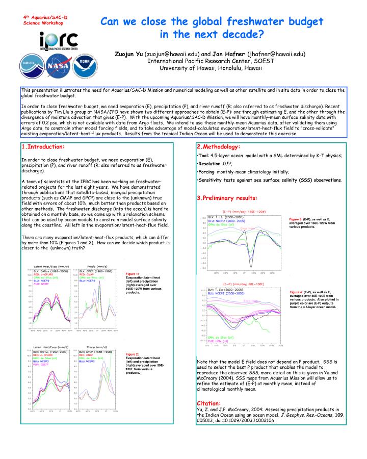
Can we close the global freshwater budget in the next decade?. 4 th Aquarius/SAC-D Science Workshop. Zuojun Yu ( zuojun@hawaii.edu) and Jan Hafner ( jhafner@hawaii.edu) International Pacific Research Center, SOEST University of Hawaii, Honolulu, Hawaii.

E N D
Can we close the global freshwater budget in the next decade? 4th Aquarius/SAC-D Science Workshop Zuojun Yu(zuojun@hawaii.edu) and Jan Hafner (jhafner@hawaii.edu) International Pacific Research Center, SOEST University of Hawaii, Honolulu, Hawaii This presentation illustrates the need for Aquarius/SAC-D Mission and numerical modeling as well as other satellite and in situ data in order to close the global freshwater budget. In order to close freshwater budget, we need evaporation (E), precipitation (P), and river runoff (R; also referred to as freshwater discharge). Recent publications by Tim Liu's group at NASA/JPO have shown two different approaches to obtain (E-P): one through estimating E, and the other through the divergence of moisture advection that gives (E-P). With the upcoming Aquarius/SAC-D Mission, we will have monthly-mean surface salinity data with errors of 0.2 psu, which is not available with data from Argo floats. We intend to use these monthly-mean Aquarius data, after validating them using Argo data, to constrain other model forcing fields, and to take advantage of model-calculated evaporation/latent-heat-flux field to "cross-validate" existing evaporation/latent-heat-flux products. Results from the tropical Indian Ocean will be used to demonstrate this exercise. • Introduction: • In order to close freshwater budget, we need evaporation (E), precipitation (P), and river runoff (R; also referred to as freshwater discharge). • A team of scientists at the IPRC has been working on freshwater-related projects for the last eight years. We have demonstrated through publications that satellite-based, merged precipitation products (such as CMAP and GPCP) are close to the (unknown) true field with errors of about 10%, much better than products based on other methods. The freshwater discharge (into the ocean) is hard to obtained on a monthly base, so we came up with a relaxation scheme that can be used by ocean models to constrain model surface salinity along the coastline. All left is the evaporation/latent-heat-flux field. • There are many evaporation/latent-heat-flux products, which can differ by more than 10% (Figures 1 and 2). How can we decide which product is closer to the (unknown) truth? • 2.Methodology: • Tool: 4.5-layer ocean model with a SML determined by K-T physics; • Resolution: 0.5o; • Forcing: monthly-mean climatology initially; • Sensitivity tests against sea surface salinity (SSS) observations. • 3.Preliminary results: • Note that the model E field does not depend on P product. SSS is used to select the best P product that enables the model to reproduce the observed SSS; more detail on this is given in Yu and McCreary (2004). SSS maps from Aquarius Mission will allow us to refine the estimate of (E-P) at monthly mean, instead of climatological monthly mean. • Citation: • Yu, Z. and J.P. McCreary, 2004: Assessing precipitation products in the Indian Ocean using an ocean model. J. Geophys. Res.-Oceans, 109, C05013, doi:10.1029/2003JC002106. Figure 3: (E-P), as well as E, averaged over 160E-120W from various products. Figure 1: Evaporation/latent heat (left) and precipitation (right) averaged over 160E-120W from various products. Figure 4: (E-P), as well as E, averaged over 50E-100E from various products. Also plotted in purple color are (E-P) outputs from the 4.5-layer ocean model. Figure 2: Evaporation/latent heat (left) and precipitation (right) averaged over 50E-100E from various products.