Download

1 / 31
310 likes | 493 Views
variables. > a = 24 > b<-25 > sqrt(a+b) > a = "The dog ate my homework" > sub("dog","cat",a) > a = (1+1==3) > a. numeric. character string. logical. variables. paste("X", "Y") paste("X", "Y", sep = " + ") paste("Fig", 1:4) paste(c("X", "Y"), 1:4, sep = "", collapse = " + ")

E N D
variables > a = 24 > b<-25 > sqrt(a+b) > a = "The dog ate my homework" > sub("dog","cat",a) > a = (1+1==3) > a numeric character string logical
variables paste("X", "Y") paste("X", "Y", sep = " + ") paste("Fig", 1:4) paste(c("X", "Y"), 1:4, sep = "", collapse = " + ") x<-2.17 y<-as.character(x) z<-as.numeric(y) a = c(1,2,3) a*2
Vector/list a = c(7,5,1) a[2] doe = list(name="john",age=28,married=F) doe$name
id<-c("xx348", "xx234", "xx987") locallization<-c("proximal", "distal", "proximal") progress<-c(F, T, F) tumorsize<-c(6.3, 8.0, 10.0) results<-data.frame(id, locallization , tumorsize, progress) > results id locallization tumorsize progress 1 xx348 proximal 6.3 FALSE 2 xx234 distal 8.0 TRUE 3 xx987 proximal 10.0 FALSE
results[3,2] results[1,] results[c(1,3),] results[c(T,F,T),] results$locallization results[ results$locallization=="proximal", ] > results id locallization tumorsize progress 1 xx348 proximal 6.3 FALSE 2 xx234 distal 8.0 TRUE 3 xx987 proximal 10.0 FALSE
x = c(1, 1, 2, 3, 5, 8) x[c(TRUE, TRUE, FALSE, FALSE, TRUE, TRUE)] x[c(TRUE, FALSE)] x == 1 x[x == 1] x[x%%2 == 0] y = c(1, 2, 3) y[]=3 y
a=matrix(1:9, ncol = 3, nrow = 3) a b=matrix(c(TRUE, FALSE, TRUE), ncol = 3, nrow = 3) b x=1:10 y=11:20 z=matrix(c(x,y)) z z=matrix(c(x,y),nrow=2) z z=matrix(c(x,y),nrow=4) z
R code max(z) min(z) length(z) mean(z) sd(z) sum(z)
expression<-factor(c("over","under","over","unchanged","under","under"))expression<-factor(c("over","under","over","unchanged","under","under")) levels(expression) expression[6]="x" expression
Working directory setwd("D:/data") x<-read.table("profiles.csv", sep=",", header=TRUE) matplot(x, type="l") matplot(x, type="l", xlab="fraction", ylab="quantity", col=1:6, lty=1:5, lwd=2) write.table(x, file="test.txt", sep="\t")
xmax<-apply(x, 2, max) xmax ymax<-apply(x, 1, max) ymax Apply the max function on columns (2) or rows (1) of matrix x
Legend matplot(x,type="l",xlab="fraction",ylab="quantity",col=1:6,lty=1:5, lwd=2) legend(x=600,legend=names(x),col=1:6,lty=1:5,lwd=2,bg="snow")
> x • x p1 p2 p3 p4 p5 p6 p7 p8 p9 p10 p11 p12 • 1 0 148 6 5 197 1 12 9 0 4 0 11 0 • 2 4 185 5 9 180 73 6 5 1 5 12 15 3 • 3 11 149 177 282 446 400 7 7 3 0 8 223 2 • 4 29 103 210 299 1264 912 3 599 2 2 6 865 387 • 5 7 72 131 197 520 171 181 301 411 864 561 266 763 • 1 75 7 11 125 34 241 1222 611 1175 216 133 511 • xmax <- apply(x, 2, max) • xscaled = scale(x, scale=xmax, center=FALSE)
Writing a Program • Can save a file as do in perl • Use “source” command to load the file
setwd("D:/data") x<-read.table("profiles.csv", sep=",", header=TRUE) xmax <- apply(x, 2, max) xscaled = scale(x, scale=xmax, center=FALSE) matplot(xscaled, type="l") Write this to a file named “profile.r” and save to D:\data
setwd("D:/data") source("profile.r") Write this to a file named “profile.r” and save to D:\data
Function • Functions in R are dened using the function keyword. Curly braces are used to dene the body of the function. • The value / object returned by the function is indicated by the return keyword.
square = function(x) { return(x^2) } z=square(4) z
plus= function(x,y) { return(x+y) } z=plus(4,5) z
z=10 z=sqrt(z) if (z<5) print("<5") else if (z == 5) print ("z==5") else print("z>5")
evenodd = function(x) { if (!is.numeric(x)) { print("neither") } else if (x%%2 == 0) { print("even") } else { print("odd") } } evenodd(10)
Loop • for • while • repeat
for (x in 1:3) { print(x) } for (x in c("hello", "goodbye")) { print(x) }
for (x in 1:4) { if (x%%2==0) next print(x) } for (x in 1:3) { if (x==2) break print(x) }
#test x = 1 while (x < 3) { print(x) x = x + 1 }
cars <- c(1, 3, 6, 4, 9) plot(cars) barplot(cars) suvs <- c(4,4,6,6,16) hist(suvs) pie(suvs)
x <- c(1,3,6,9,12) y <- c(1.5,2,7,8,15) plot(x,y) myline.fit <- lm(y ~ x) abline(myline.fit) x2 <- c(0.5, 3, 5, 8, 12) y2 <- c(0.8, 1, 2, 4, 6) points(x2, y2, pch=16, col="green")
d<-dist(t(xscaled),method="euclidean") dendrogram=hclust(t(d),method="complete",members=NULL) plot(dendrogram) rect(1,0,2,1)
cummean = function(x){ n = length(x) y = numeric(n) z = c(1:n) y = cumsum(x) y = y/z return(y) } n = 10000 z = rnorm(n) x = seq(1,n,1) y = cummean(z) X11() plot(x,y,type= 'l',main= 'Convergence Plot')