Download
1 / 29
290 likes | 477 Views
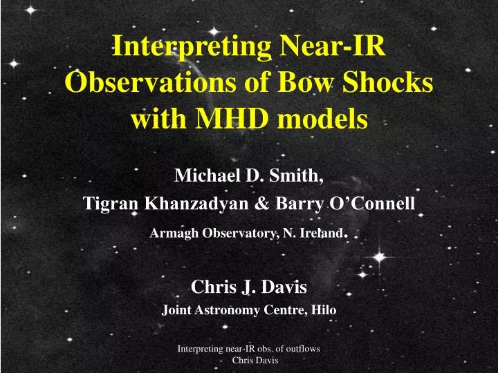
Interpreting Near-IR Observations of Bow Shocks with MHD models. Michael D. Smith, Tigran Khanzadyan & Barry O’Connell Armagh Observatory, N. Ireland . Chris J. Davis Joint Astronomy Centre, Hilo. Bow Shocks in Star Forming Regions. Sometimes isolated, sometimes part of a collimated flow

E N D
Interpreting Near-IR Observations of Bow Shocks with MHD models Michael D. Smith, Tigran Khanzadyan & Barry O’Connell Armagh Observatory, N. Ireland. Chris J. Davis Joint Astronomy Centre, Hilo Interpreting near-IR obs. of outflows - Chris Davis
Bow Shocks in Star Forming Regions... • Sometimes isolated, sometimes part of a collimated flow • Symmetry axis, luminosity, motion :- head of a supersonic jet or dense clump • Line ratios :- gas excited by shock waves • Flow impacts ambient or internal shocks (momentum transfer, physics, history of flow…) Interpreting near-IR obs. of outflows - Chris Davis
Bow shocks in outflows from the youngest stars... H2 - a powerful tracer… • Imaging (morphology, proper motions) • Low-resolution Spectroscopy (excitation) • Echelle spectroscopy (kinematics)
HH 7 and L 1634 (HH 240-241) Smith, Khanzadyan & Davis (2003), MNRAS, 339, 524 O’Connell et al. (2004), A&A, submitted HH 7-11 HH 240 Interpreting near-IR obs. of outflows - Chris Davis
HH7 - the observations • Narrow, flattened ridge • Ring of emission (central hole?) • [FeII] (and [SII]) ‘behind’ H2 ridge and hole… (Stapelfeldt et al. 1991) Interpreting near-IR obs. of outflows - Chris Davis
HH7 - the observations Constant, low, overall 2-1/1-0 ratio ~ 0.1 Interpreting near-IR obs. of outflows - Chris Davis
HH7 - the observations Double peaked - emission from bow and jet?? -100 km/s 0 km/s Interpreting near-IR obs. of outflows - Chris Davis
HH 240 observations Michael D. Smith, Tigran Khanzadyan & Barry O’Connell Armagh Observatory, N. Ireland. Interpreting near-IR obs. of outflows - Chris Davis
HH 240 observations Changing 1-0/2-1 ratio through bow A and C… Excitation lower in flanks
HH 240 observations • Gas generally blue by 10-50 km/s • Wide-ish profiles, 70 km/s • Broader profiles at bow heads, narrower in flanks... 100 km/s Interpreting near-IR obs. of outflows - Chris Davis
The Modeling… C- or J-shock ?? For molecular emission, the main choice is between J-shock and C-shock physics... (Hollenbach 1997) • J-shock: steep wave, impulsive heating and acceleration. Vsh > 25 km/s, molecules dissociated. Rapid cooling; radiative zone which provides (weak) molecular emission. (Emission from reformation region, at 500 K, negligeable.) • C-shock: transfer of momentum mediated by ions. If ion fraction low, ions can diffuse ahead of shock and ‘communicate its arrival’. Gas more gradually accelerated and heated; lower heating rate & heating over greater distance = stronger IR emission from molecules. Interpreting near-IR obs. of outflows - Chris Davis
The Modeling… C- or J-shock ?? Previous modeling favours C-shock FOR H2 EMISSION REGION, since: 1. J-shocks predict higher excitation, 2-1S(1)/1-0s(1) > 0.2 which is rarely observed: Need extended flanks to get bright, low-excitation emission; but we don’t usually see these flanks in the images. 2. Line widths are limited to < 2x Vdissoc ~50 km/s Interpreting near-IR obs. of outflows - Chris Davis
The Modeling… C- or J-shock ?? J-shock and C-shock physics... H2 (2.12um) - red [FeII] (1.64um) - green [SII] (0.66um) - blue C-shock if alfven speed exceeds the shock speed, giving rise to a magnetic precursor... Interpreting near-IR obs. of outflows - Chris Davis
Bow model for H2 in HH 7 and HH 240 For simplicity: 1. Parameterise the geometry of the bow shock. Surface of revolution, z/d = 1/s (R/d)s, where s is the shape, d is scale length (cylindrical coords). s=2 ; parabola; s=1 conic. 2. Treat each element of the bow surface as a planar shock 3. Assume homogeneous pre-shock medium, with uniform B-field (though orientation of B is a variable) 4. Limit time dependent chemistry to H, H2, C and O But also...: 1. No longer assume cooling length and shock thickness negligible w.r.t. overall bow shape. Now include distance travelled by shocked gas.
Bow models for H2 emission regions A few generalities (to bear in mind)... 1. The bow velocity determines the location of the H2 emission. 2. Orientation influences observed structure (obviously) 3. The hydrogen density and bow speed dictate total power, line intensities and cooling lengths 4. Ion fraction and B-field affect shock thickness and dissociation speed limit. (Hence, first determine density from line flux, then ion fraction and B-field strength.) 5. C and O abundances varied to match available obs (e.g. ISO). 6. Instabilities not considered… (probably important)
Heating/Cooling functions • Gas-grain (dust) cooling • Collisional cooling from H2 molecules - rotational/vibrational • Collisional cooling from atoms • Collisional cooling from water - rotational and vibrational - from collisions with H2 and H • Dissociation of H2 - cooling • Collisional cooling from CO - rotational and vibrational - from collisions with H2 and H • [OI] fine structure cooling • [CI] fine structure cooling • OH cooling • Heating from reformation of H2 Limited non-equilibrium chemistry is included, involving O, OH, C, CO, H2O (from Smith & Rosen 2002)
HH 7 Synthetic images - shape parameter, s... s = 1.5 s = 2.5 Interpreting near-IR obs. of outflows - Chris Davis
HH 7 Synthetic images - orientation... 15o to line of sight 45o to line of sight Interpreting near-IR obs. of outflows - Chris Davis
HH 7 Synthetic images - bow velocity... 30o to line of sight 30 km/s 30o to line of sight 80 km/s Interpreting near-IR obs. of outflows - Chris Davis
Model parameters... • Bow speed 55 km/s (no UV/fluorescent contribution…) • Hydrogen density 8x103 cm-3 • B=10-4 G (Alfven speed ~ 2 km/s) • Ion fraction = 2x10⁻⁶ • 1-0S(1) & 2-1S(1) emission peaks coincident, so oblique orientation (30o to line-of-sight). Ratio of 0.15 predicted; 0.10 is observed (extinction?) • Low density (and low H2 fraction; 20%) yields observed 1-0S(1) flux.
Velocity structure (echelle observations) Jet shock! -12 km/s (w.r.t systemic) -5 km/s (w.r.t systemic) -100 km/s 0 km/s -11 km/s -4 km/s Profile smoothed with 8 km/s gaussian (resoln. Of observations)
HH 7 What about a J-bow shock model ??? • 30o to line of sight. • 40 km/s (Vsh lower to keep emission near bow head). • Higher radial velocities. • 2-1/1-0 ~ 0.2 (too high). Interpreting near-IR obs. of outflows - Chris Davis
HH 240 modeling Parameter HH 240A HH240C angle 60degs 60degs velocity 70km/s 50km/s s 2.35 1.90 density 2.5e3 7e3 ion frac 1e-5 5e-5 B-field 0.1e-3G 0.2e-3G • In HH 240C, non-dissociative cap; lower bow speed • Shape parameter s lower in 240C - more pointed, conical morphology • 240C as luminous as 240A; smaller, so higher density needed • 240C higher excitation than 240A - again, higher density needed
HH 240 A Synthetic images - asymmetries? m = 45o m = 30o Interpreting near-IR obs. of outflows - Chris Davis
HH 240 C Synthetic images - asymmetries? C-bow; m = 60o J-bow; Vsh = 42 km/s Den. = 2.104 cm-3 Ion frac . > 10-4 But high excitation in this object, 2-1/1-0 ~ 0.2: J-shock for 240C ? Interpreting near-IR obs. of outflows - Chris Davis
Slit 1 (bottom) Slit 2 (top) HH 240AVelocity structure (echelle observations) C-bow model 100 km/s -11 km/s -4 km/s Profile smoothed with 8 km/s gaussian (resolution of observations)
C-bow model HH 240C Slit 5 (middle) 70 km/s J-bow model HH 240C J-bow: Narrower H2 lines predicted. Must be less than 2vdsinq ~ 43 km/s.
Excitation from long-slit spectra… (Data - Nisini et al. 2002) • Lines from v=1 (squares),v=2 (crosses) and v=3 (triangles) fit separately • HH240A - good fit • HH240C - slightly better fit with J-bow to higher-energy lines (vibrational levels closer to LTE) C-bow C-bow J-bow
Conclusions • Bow-shock models yield good fits to morphologies, velocities and excitation (with reasonable parameters!) • Given high-enough resolution and enough data, we can distinguish J- from C-shocks... • C- and J-type shock physics can exist in the same flow, and even in the same bow shock. Interpreting near-IR obs. of outflows - Chris Davis