Molecular Control Engineering Nonlinear Control at the Nanoscale

1. Molecular Control Engineering Nonlinear Control at the Nanoscale Raj Chakrabarti PSE Seminar Feb 8, 2013

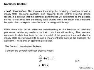
2. What is Molecular Control Engineering? • Control engineering: Manipulation of system dynamics through nonequilibrium • modeling and optimization. Inputs and outputs are macroscopic variables. • Molecular control engineering: Control of chemical phenomena through microscopic • inputs and chemical physics modeling. Adapts to changes in the laws of Nature at these length and time scales. • Aims • Reaching ultimate limits on product selectivity • Reaching ultimate limits on sustainability • Emulation of and improvement upon Nature’s strategies

3. Approaches to Molecular Design and Control Quantum Control of Chemical Reaction Dynamics Control of Biochemical Reaction Networks Static Optimization Molecular Design [protein pic] milliseconds, micrometers femtoseconds, angstroms picoseconds, nanometers

4. Parallel Parking and Nonlinear Control • Stepping on gas not enough: can’t move directly in direction of interest • Must change directions repeatedly • Left, Forward + Right, Reverse enough in most situations • Tight spots: Move perpendicular to curb through sequences composed of Left, Forward + Left, Reverse + Right, Forward + Right, Reverse

5. Vector Fields 8. Finalize these

6. Control with Linear Vector Fields

7. Lie Brackets and Directions of Motion

8. From classical control to the coherent control of chemical processes • FMO photosynthetic protein complex transports solar energy with ~100% efficiency • Phase coherent oscillations in excitonic transport: exploit wave interference • Biology exploits changes in the laws of nature in control strategy: can we?

10. Coherent Control versus Catalysis • Potential Energy Surface • with two competing • reaction channels • Saddle points separate • products from reactants • Dynamically reshape • the wavepacket traveling on the • PES to maximize the probability • of a transition into the desired • product channel probability density time interatomic distance

11. C. Brif, R. Chakrabarti and H. Rabitz, New J. Physics, 2010. C. Brif, R. Chakrabarti and H. Rabitz, Control of Quantum Phenomena. Advances in Chemical Physics, 2011.

12. Femtosecond Quantum Control Laser Setup 2011: An NSF funded quantum control experiment collaboration between Purdue’s Andy Weiner (a founder of fs pulse shaping) and Chakrabarti Group

13. Prospects and Challenges for Quantum Control Engineering

14. Coherent Control of State Transitions in Atomic Rubidium http://www.lamptech.co.uk

15. Bilinear and Affine Control Engineering R. Chakrabarti, R. Wu and H. Rabitz, Quantum Multiobservable Control. Phys. Rev. A, 2008. Possibly move one of these below

16. Few-Parameter Control of Quantum Dynamics • Conventional strategies based on excitation with resonant frequencies fails to achieve maximal population transfer to desired channels • Selectivity is poor; more directions of motion are needed to avoid undesired states

17. Optimal Control of Quantum Dynamics • Shaped laser pulse generates all directions necessary for steering system toward target state • Exploits wave-particle duality to achieve maximal selectivity, like coherent control of photosynthesis

18. Understanding Interferences Need to introduce V_I Remove the lambdas We don’t show the intermediate states here; should we for consistency w below? 9. Finalize these

19. Quantum Interferences and Quantum Steering i is part of v • Mechanism identification techniques have been devised to efficiently extract important constructive and destructive interferences Interference V. Bhutoria, A. Koswara and R. Chakrabarti, Quantum Gate Control Mechanism Identification, in preparation

20. Control of Molecular Dynamics HCl Would need to define rho, O, mentioning Boltzmann, with Pif case indicated (get above eqns from book slides, now that removed from slide above), show GR figs regarding scaling w examples of rhos; then this fig on topology with the eqns from the next slide CO Mixed state density matrix: Pure state: \begin{equation}\label{kincost} J(\varepsilon(\cdot))= F_1(\psi_T) = Tr(\rho_T \Theta) = \langle \psi_T| \Theta | \psi_T \rangle, \end{equation} Expectation value of observable: Cost functional: R. Chakrabarti, R. Wu and H. Rabitz, Quantum Pareto Optimal Control. Phys. Rev. A, 2008. 2. Do in mathtype since figs needed; start by prepping beamer code; paste figs here

21. Quantum System Learning Control: Critical Topology R. Wu, R. Chakrabarti and H. Rabitz, Critical Topology for Optimization on the Symplectic Group. J Opt. Theory, 2009 R. Chakrabarti and H. Rabitz, Quantum Control Landscapes, Int. Rev. Phys. Chem., 2007 K.W. Moore, R. Chakrabarti, G. Riviello and H. Rabitz, Search Complexity and Resource Scaling for the Quantum Optimal Control of Unitary Transformations. Phys. Rev. A, 2011.

22. Quantum Robust Control R. Chakrabarti and A. Ghosh. Optimal State Estimation of Controllable Quantum Dynamical Systems. Phys. Rev. A, 2011.

23. Improving quantum control robustness Check sign, fix index

24. May omit one of these slides

25. From Quantum Control to Bionetwork Control • Nature has also devised remarkable catalysts through molecular design / evolution • Maximizing kcat/Km of a given enzyme does not always maximize the fitness of a network of enzymes and substrates • More generally, modulate enzyme activitiesin real time to achieve maximal fitness or selectivity of chemical products

26. The Polymerase Chain Reaction: An example of bionetwork control Nobel Prize in Chemistry 1994; one of the most cited papers in Science (12757 citations in Science alone) Produce millions of DNA molecules starting from one (geometric growth) Used every day in every Biochemistry and Molecular Biology lab ( Diagnosis, Genome Sequencing, Gene Expression, etc.) Generality of biomolecular amplification: propagation of molecular information - a key feature of living, replicating systems March 2005: Roche Molecular Diagnostics PCR patents expire 2007: Celera Licenses and Roche negotiates for Chemical PCR patents

27. DNA Melting Again Single Strand – Primer Duplex Extension DNA Melting Primer Annealing 9/3/2014 School of Chemical Engineering, Purdue University 27

28. The DNA Amplification Control Problem and Cancer Diagnostics Mutated DNA Wild Type DNA • Can’t maximize concentration of target DNA sequence by maximizing any individual kinetic parameter • Analogy between a) exiting a tight parking spot • b) maximizing the concentration of one DNA sequence in the presence of single nucleotide polymorphisms

29. PCR Temperature Control Model Sequence-dependent annealing DNA targets Cycling protocol

30. Sequence-dependent Model Development Reaction Equilibrium Information ΔG – From Nearest Neighbor Model Relaxation Time Similar to the Time constant in Process Control τ – Relaxation time (Theoretical/Experimental) Solve above equations to obtain rate constants K. Marimuthu and R. Chakrabarti, Sequence-Dependent Modeling of DNA Hybridization Kinetics: Deterministic and Stochastic Theory, in preparation

31. Sequence-dependent rate constant prediction • σ – Nucleation constant for resistance to form the first base pair • The forward rate constant is a fixed parameter • Estimate σ, forward rate constant offline based on our experimental data • Compute t and hence kf, kr for a given DNA sequence using Reaction Mechanism • Sequence dependence comes from s_i = ki-1 /ki+1 - Stability constant for • each base pair formation – Can be obtained from known NN parameters. S. Moorthy, K. Marimuthu and R. Chakrabarti, in preparation

32. Variation of rate constants Leave this in terms of just one primer?

33. Flow representation of standard PCR cycling Insert comments on parallel parking analogy, Lie brackets from above Choose times

34. The \emph{reachable set} from point $p \in X$ at time $t$ is a submanifold of the state space $X$ Now parameterizing vector fields by controls $u$ (manipulated inputs), From standard to generalized PCR cycling Accessibility May mention reachable set here rather than above May remove / send to backup 6. Decide what to show, finalize Specify controls in finite set • Reachable set May show affine extension state equations in u,f,g format Then transition to full OCT – for nonlinear problem, application of vector fields in arbitrary combinations PCR gradient, mentioning PMP and definition of \phi(t) (can then indicate below that gradient components in 2nd cycle will be ~ null) Project flow w Gramian in terms of \phi(t) – for comments on model-free learning control of competitive problems below)

35. Optimal Control of DNA Amplification For N nucleotide template – 2N + 13 state equations Typically N ~ 103 R. Chakrabarti et al. Optimal Control of Evolutionary Dynamics, Phys. Rev. Lett., 2008 K. Marimuthu and R. Chakrabarti, Optimally Controlled DNA amplification, in preparation

36. Optimal control of PCR

37. Optimal control of PCR Minimal time control? Apply Lagrange cost

38. Optimal control of PCR

39. Optimal control of PCR Competitive problems? Check rank of Gramian

40. Optimal control of PCR Cycle 1 Cycle 2 Geometric growth: after 15 cycles, DNA concentrations are red – 4×10-10 M blue – 8×10-9 M green – 2×10-8 M

41. Technology Development for Control of Molecular Amplification • Next steps: application of nonlinear programming dynamic • optimization strategies for longer sequences, competitive • problems • Future work: robust control, real-time feedback control using parameter distributions we obtain from experiments

42. Summary • Can reach ultimate limits in sustainable and selective chemical engineering through advanced dynamical control strategies at the nanoscale • Requires balance of systems strategies and chemical physics • New approaches to the integration of computational and experimental design are being developed

43. Reviews of our work Quantum control • R. Chakrabarti and H. Rabitz, “Quantum Control Landscapes”, Int. Rev. Phys. Chem., 2007 • C. Brif, R. Chakrabarti and H. Rabitz, “Control of Quantum Phenomena” New Journal of Physics, 2010; Advances in Chemical Physics, 2011 • R. Chakrabarti and H. Rabitz, Quantum Control and Quantum Estimation Theory, Invited Book, Taylor and Francis, in preparation. Bionetwork Control and Biomolecular Design • “Progress in Computational Protein Design”, Curr. Opin. Biotech., 2007 • “Do-it-yourself-enzymes”, Nature Chem. Biol., 2008 • R. Chakrabarti in PCR Technology: Current Innovations, CRC Press, 2003. • Media Coverage of Evolutionary Control Theory: The Scientist, 2008. Princeton U Press Releases

45. \item The Campbell-Baker-Hausdorff formula(s) provides... \begin{align*} \exp(A)\exp(B)&=\exp(A+B+\frac{1}{2!}[A,B]+\frac{1}{12}[A,[A,B]]+\frac{1}{12}[B,[A,B]]\cdots\\ \end{align*} \item Application of the CBH formula to a bilinear control system $$\frac{dy}{dt}=H(t)y(t)=(A+u(t)B(t))y(t)$$ gives \begin{align*} \mathbb{T}\exp\left\{\int_0^t H(t')~dt'\right\} &= \exp\biggr\{ \int_0^t H(t')~dt'+\frac{1}{2!}\int_0^t \int_0^{t'}\left[H(t'), H(t'')\right]~dt"dt' +\\ &\frac{1}{12}\int_0^t\int_0^{t'} \int_0^{t'} \left[H(t'), \left[H(t"), H(t''')\right]\right]~dt'''dt"dt' + \cdots \end{align*} where $\mathbb{T}$ denotes the time-ordering operator \item In quantum control, $H(t) = -i(H_0 - \mu\e(t))$, where $H_0$ and $\mu$ are Hermitian matrices • Insert more slides here: • A) Affine control system (edit slide above to precede bilinear w affine?) • B) possibly Magnus expansion vis-à-vis controllability. Possibly geometric picture of Lie brackets, Ad formula vis-à-vis CBH Simplify – may show only magnus, or completely avoid it since we will be showing Dyson later. Could use beamer decide last

46. Pathway Examples • 6 level system, Pif transition • (i) Amplitude of 2nd order pathway via state 2: • (ii) Transition amplitude for 3rd order pathway (i) (ii)

47. Normal H(t) Uba(T) Dynamics Encode Decode {Unba} Encoded H(t,s) Uba(T,s) Dynamics Interference Identification Fix for composite pathways, or redo slide for orders Must show example of MI inverse FFT w arrow pointing to an n-th order pathway

48. Linear Programming Formulation: Observable Max • Quantum observable maximization: • Translation to linear programming: Mention riemannian geometry working paper K. Moore, R. Chakrabarti, G. Riviello and H. Rabitz, Search Complexity and Resource Scaling for Quantum Control of Unitary Transformations. Phys. Rev. A, 2010 .

49. The analogy to the “assignment problem” • Maximum weighted bipartite matching (assignment prob): Given N agents and N tasks Any agent can be assigned to perform any task, incurring some cost depending on assignment Goal: perform all tasks by assigning exactly one agent to each task so as to maximize/minimize total cost

50. Foundation for Quantum System Learning Control. II: Geometry of Search Space R. Chakrabarti and R. Wu, Riemannian Geometry of the Quantum Observable Control Problem • Maximum weighted bipartite matching of \gamma_i,\lambda_j • Birkhoffpolytope: • flows start from points within polytopes and proceed to optimal vertex 5. Maximum weighted bipartite matching (assignment prob):Would need to mention Birkhoff polytope and then indicate the two examples shown in notes in a separate slide, then show projected flow on polytope in terms of just one matrix G_thick, indicate it is inverse metric due to compatibility cond’n, and indicate in bullet point that flows start from points within polytopes and proceed to optimal vertex (do not need to draw the polytopes now) Replace w polytope formulation M: inverse Gramian, Riemannian metric on polytope R. Chakrabarti and R.B. Wu, Riemannian Geometry of the Quantum Observable Control Problem, 2013, in preparation.