Download
1 / 24
280 likes | 551 Views
Ashfaq Ahmad On behalf of the ATLAS collaboration Stony Brook University 11th ICATPP, Villa Olmo 5-9 October 2009, Como Italy. Electron and Photon Reconstruction and Identification with the ATLAS Detector. Electrons and photons @ LHC.

E N D
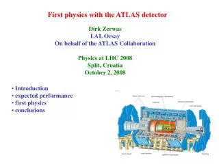
Ashfaq Ahmad On behalf of the ATLAS collaboration Stony Brook University 11th ICATPP, Villa Olmo 5-9 October 2009, Como Italy Electron and Photon Reconstruction and Identification with the ATLAS Detector
Electrons and photons @ LHC • At the LHC electrons and photons are expected to be produced in many physics channels of interest • And within a large energy range, typically from few GeV to 5 TeV • Some important sources of Electrons/photons: • Electrons from J/, Y, W and Z bosons decays • Non-isolated electrons from heavy flavor decays • Used for performance studies and detector calibration, also above is background to new physics • Electrons from higgs decay, e.g. HZZ*4e • BSM: electrons form Z’ decay, SUSY and extra dimensions • Isolated photons from H and G • But a lot of background; e.g. Electron to QCD jet ratio~10-5 with pT from 20-50 GeV • Requires excellent electron/photons reconstruction and identification capability Ashfaq Ahmad
Object Reconstruction Will discuss this part Ashfaq Ahmad
Inner Detector (Tracker) Inner Detector: • Pixel : • barrel - 3 layers, 67M pixels • end-cap – 3 layers 6.6M pixels • SCT (Semi Conductor Tracker): • barrel - 8 layers, ~2M channels • end-cap – 9 layers, ~2M channels • TRT (Transition Radiation Tracker) • barrel - 73 layers, ~53k channels • end-cap - 160 layers, ~123k channels • Inside 2 Tesla Solenoid • Precision tracking for pT > 0.5 GeV inside ||<2.5 • Tracker radiation length ~0.5-1.5 • Relative transverse momentum resolution~1.5-4% for 20-100GeV tracks in the barrel Ashfaq Ahmad
Liquid Argon (LAr) Calorimeter 2 X0 16 X0 4.3 X0 • Good energy resolution: • With b=sampling term~10%/E • a= noise term~0.3GeV and ctot ~0.7% Coverage, ||<3.2 Ashfaq Ahmad
Electron/Photons reconstruction • Algorithms: • Calorimeter seeded (Standard egamma): • Starts from reconstructed clusters in the EM calorimeter, match cluster with tracks in the Inner detector (tracker) within a window x =0.05x0.1 and E(cluster)/P<10 • To determine if particle is electron (track match), photon (no track) or converted photon (with associated conversion) • Early classification allows to apply different corrections to electrons and photons • Build identification variables based on EM calorimeters and inner detector • Used for high pT isolated electrons/photons • Track seeded algorithm (Soft-electron reconstruction): • Starts from good-quality tracks in the tracker, matching with energy deposition in calorimeter • Build identification variables as above • Used mainly for low pT electrons up to few GeV e.g. electrons from J/ and b and c quarks Ashfaq Ahmad
Calibration/correction steps Cell-Level Calibration Cluster level Calibration In situ Calibration Electron reconstruction Absolute scale Intercalibration Raw signalenergy deposit MC based calibration Calibration loop Cluster corrections steps How to combine energy deposited in each layer Ashfaq Ahmad
Clustering algorithm • Electrons/photons deposit energy in many calorimeter cells • Clustering algorithms group cells together and sum the total deposited energy within each cluster • Energies are calibrated to account for energy deposited outside the cluster and dead material • Sliding-Window algorithm: • Build a pre-cluster using a fixed size 5x5window (seed) of cells • The 5x5 window is moved over the tower grid • Position of the window is adjusted so to contain a local maximum in energy • A threshold of 3 GeV on transverse energy is applied • Build clusters of different sizes based on particle type and calorimeter region • Apply cluster calibrations photon 3x5 Endcap, all types 5x5 Converted photon 3x7 Electron 3x7 Ashfaq Ahmad
Cluster calibration: energy reconstruction • Combine energy deposits in each layer and the presampler • Compute corrections by using special simulations (Calibration Hits) where energy deposited in all material (active + inactive) is recorded • Energy depositions in the inactive material can be correlated with the measurable quantities • Corrections are derived for electrons and photons separately Calib. factor vs X Electron=solid Photon =open X = Shower depth Xi = long. depth of layer “i” Ei = energy deposit in layer “i” Sacc(X,) = calib. factor Ashfaq Ahmad
Performance (linearity and resolution) Energy resolution • At low resolution similar for electron and photon • At large resolution worse for electron due to more material • Sampling term for electron goes from~9% at low to ~21% at high • For photons maximum sampling term~12% • constant term < 0.6% • linearity within 0.5% for both electron and photons for energies from 25-500GeV ||=0.3 Energy resolution Linearity, photon ||=1.65 Ashfaq Ahmad
Electron/Photon Identification • Efficient electron/photon identification methods are needed to reject huge QCD background • Several methods developed in ATLAS namely; • Cut-based identification (Standard) • Multivariate techniques: • Log-likelihood ratio based identification • Covariance-matrix-based identification (H-matrix) • Boosted decision tree and neural network techniques • Here I’ll discuss cut-based identification • Discriminating variables used for electron/photon Id. and jet rejection • Hadronic leakage (Ehad1/Eclus) • Shower shape in the middle layer of EM calorimeter • Shower shape in the strip layer (search for 2nd maximum for 0 rejection) • Isolation in calorimeter • Track isolation to reject low track multiplicity jets containing 0 • Variables used for Electron Only: • Track quality (# of hits, impact parameter) • Track match • Fraction of high threshold TRT hits Ashfaq Ahmad
Identification of Electron and Photon (discriminating variables) Signal: H Background: QCD jets Signal: H Background: QCD jets In first layer (strips) Es =Emax2 - Emin Signal(blue): Zee Background: QCD di-jets Signal: H Background: QCD jets Middle layer E2(3x7)/E2(7x7) Middle layer E2(3x3)/E2(3x7) Ashfaq Ahmad
Performance of the cut-based Identification (electron) • Three sets of identification cuts are defined by combining discriminating variables discussed before • Namely; Loose, medium and tight cuts • Electron identification efficiency in Heeee decays H4e pT > 5GeV H4e pT > 5GeV | | ET (GeV) Recent work has resulted significant improvement in electron efficiency Ashfaq Ahmad
Performance of the cut-based Identification (jet rejection) • Expected differential cross section after tight cuts from W/Z, QCD di-jets and minimum bias simulated samples @ 100pb-1 • QCD hard jets with ET>17GeV • Minimum bias ET> 8GeV • Shapes of electrons from non-isolated and residual jet background are similar • ~100k electrons from b and c decays with ET >10GeV per pb-1 • ~5k electrons with ET >20GeV per pb-1 ET > 17GeV ET > 8GeV electron from W/Z Ashfaq Ahmad
Performance of the cut-based Identification (photon) Fake rate =1/jet rejection • Photons from H • ET>25GeV • QCD jet background • Overall efficiency~84% with jet rejection~8000 Efficiency vs. Efficiency vs. ET Ashfaq Ahmad
Shower shapes in middle layer with cosmic muons • Comparison of later shower shapes between cosmic data and MC • Selection: • Require EM cluster of ET > 5GeV • Additional cuts to match the difference in acceptance between data and MC • At least one Si track |d0| < 220mm with pT > 5GeV • Estrips/Ecluster > 0.1 • After selection sample has 1200 photon candidates in data (out of 3.5 million) and 2161 from MC( out of~11.7 million) • Good agreement between data and MC E2(3x3)/E2(3x7) E2(3x7)/E2(7x7) Ashfaq Ahmad
Shower shapes in strip layer • Lateral shower shapes • Fside=(E±3 -E±1)/E±1 • Different shower development between top (>0) and bottom (<0) • Good agreement between data and MC For detail cosmic results please see Christian Schmitt talk on Wednesday Fside Fside Ashfaq Ahmad
In-situ intercalibration with Zee • Energy resolution is parameterized as • From the test beam the local constant (cL) term ~0.5% • Hence the “long range” zone to zone non-uniformity (cLR) must be 0.5% • zone is =0.20.4 • In-situ calibration also has to establish absolute EM scale to an accuracy~0.1% • Long range non-uniformities can be corrected using electrons from Z boson decays • Parameterize electron energy in zone “i” as • ’s are obtained from likelihood fit by constraining the measured di-electron invariant mass to the Z boson line shape with After correction 91.42±0.03 Before correction 90.38±0.03 (fit -inj) Z line shape Ashfaq Ahmad
Data driven efficiency measurements • Need to measure efficiency from data to scale MC prediction • Use “Tag and Probe” method on Zee and J/ events: • Select one good quality electron (tag, passing set of cuts) • Constrain with Z mass • Measure the efficiency of passing cuts by second electron (probe) Measuring medium cut efficiency Efficiency vs. ET Efficiency vs. Ashfaq Ahmad
Conclusion • Understanding of the electron and photon reconstruction and identification are essential for many SM physics measurement and for new physics searches at the LHC • Different algorithms have been developed in ATLAS for this purpose and thoroughly tested with beam tests, with simulations and cosmic data • The performance of ATLAS Electromagnetic (EM) calorimeter and tracker has been extensively studied • The absolute energy scale of EM calorimeter is known to be~1% and linearity better than 0.5% for wide range of energies • The MC studies show that the reconstruction and identification efficiencies and background rejection are adequate for physics measurements Ashfaq Ahmad
Backup Slides Ashfaq Ahmad
Cluster corrections 1 cell in the middle layer • Position corrections(/ corrections): • Correct for bias in position due to the finite granularity of the readout cells • depends on particle impact point within cells • give rise to S-shape in position • a few percent difference between electrons/photons corrections • corrections are and energy dependent • position resolution for photon is~3x10⁻⁴ in strips (layer 1) and ~6x10⁻⁴ in middle (layer 2) • corrections: • correct for small bias in • resolution~ 0.5-1.5x10⁻³ 100 GeV photons Ashfaq Ahmad
Δθ is defined as the angle between the direction of the shower and the direction defined from the centre of the detector to the centre of the cluster Ashfaq Ahmad