Download
1 / 30
300 likes | 440 Views
Bayesian Probability theory in astronomy: Timing analysis of Neutron Stars. VII BSAC, Chepelare, Bulgaria, 01.06.2010 Valeri Hambaryan Astrophysical Institute and University Observatory, Friedrich Schiller University of Jena, Germany E-Mail: vvh@astro.uni-jena.de. Outline of talk.

E N D
Bayesian Probability theory in astronomy: Timing analysis of Neutron Stars VII BSAC, Chepelare, Bulgaria, 01.06.2010 Valeri Hambaryan Astrophysical Institute and University Observatory, Friedrich Schiller University of Jena, Germany E-Mail: vvh@astro.uni-jena.de
Outline of talk Introduction Method Results & Outlook
Radio Pulsar Basics • spin characterized byspin period rate of change of period P time
Pulsar Basics cont... Assumes magnetic dipole braking in a vacuum spin-down luminosity characteristic age magnetic field
The pulsar HRD • 1800 pulsarsknown • 143 pulsarswithperiodlessthan 10 ms • A wholezooofnewandintersetingobjects • --AXPs/SGRs • --CCOs • --RRATs • --INSs binary
Neutron star mass and radius linking with measurable phenomena Arzoumanian (2009)
Gravitational redshift EXO 0748 (Cottam et al. 2002) Nosecondobservationofthiskind
0.096 M / R = 0.153 ?? Unable to identify FeXV-FeXVI (Rauch,Suleimanov & Werner, 2008 ) XMM-Newton non detection (Cottam et al., 2008) Spin frequency 552Hz (Galloway et al., 2009) 0.087 Radius of RXJ1856 is R = 17 km (Trümper et al., 2004) M / R = 0.153 M_sun/km for EXO 0748?? (Cottam et al., 2002) M / R = 0.096 „ for X7 47 Tuc (Heinke et al. ,2006) „ „ for LMXRBs (Suleimanov & Poutanen, 2006) M / R = 0.089 „ for Cas A (Wyn & Heinke, 2009) M / R = 0.087 „ for RBS 1223 (Hambaryan & Suleimanov, 2010)
Method • Bayesian methodology • Bayesian Variability detection • Bayesian Periodicity search
What is a Bayesian approach? • Three-fold task: What the method is? How it works? Why it?
What the method is? • Classical approach or Sampling Statistics Given the data D, how probable is variation in the data, given model M, model parameters q, and any other relevant prior information I ? P(D|qMI) or P(D|MI) • Bayesian methodology Inverse: How probable are models or model parameters given data? P(q|DMI) or P(M|DI)
What the method is? • Bayesian approch: details Given the data D, how probable are model M, model parameters q? P(q|D,M,I) = P(q|M,I) P(D|q,M,I) | P(D|M,I) P(q|D,M,I) = Posterior probability P(D|q,M,I) = Direct probability P(q|M,I) = Prior probability
How it works? • 1. Specify the hypothesis Carefully specifying the models Mi • 2. Assign direct probailities Assign direct probabilites appropriate to data (Poisson, Bernulii,...) Assign priors for parameters for each Mi • 3. „Turn the crank“ Apply Bayes‘ Theorem to get posterior probability densty distribution • Marginalize over uninteresting parameters (some prefer to look at the peak of the posterior without marginalizing) • 4. Report the results • For comparing models: it may include, likelihood ratios, probabilities • For parameters: one might report the posterior mode, or mean and variance
Bayesian variability testing • High energy astronomy and modern equipments allow: Register arrival times of individal photons with high accuracy Time binnig technique give rise to certain difficulties: • many different binnings of the data have • to be considered • the bins must be large enough so that there • will be enough photons to provide a good • stastistical smaple • larger bins will dilute short variations & • overllooks a considerable amount of info • introduces a dependency of results on the • sizes and locations of the bin
Bayesian variability testing t l1 l2 • Observational interval T consisting • of m discrete moments of time • m = T/dt • (dt spacecraft‘s „clock tick“) • Registered n photon arrival times • D (ti,ti+1,...,ti+n-1) Compare two hypothesis • First hypothesis –constantrate Poisson process • model M1: one parameter, i.e. count rate l • Second hypothesis – two-rate Poisson process • model M2: parameters l1,l2and t • t is any point from T dividing • into two parts with length • T1 & T2at which the Poisson process • switches from count rate l1to l2
Bayesian variability testing t l1 l2 • To detect so called „change points“ Change point detection mthodology deals with sets of sequentlly ordered observations (as in time) and undertakes to determine whether the fundamental mechanism generating the observations has changed during the time the data have been gathered
Bayesian variability testing t l1 l2
Detection of periodicty and QPOs Different methods have been developed for periodicdy search: Leahy et al., 1983, ApJ, 272,256; Scargle, 1989,ApJ,343,874; Swanepoel & De Beer, 1990, ApJ,350,754; Gregory & Loredo (GL), 1992, ApJ,398,146; Bai, 1992, ApJ, 397,584; Cincotta et al., 1995, ApJ, 449,231; Cicuttin et al., 1998, ApJ,498,666 , De Jager 2001.... Simple model of rotating NS • Epoch folding Fi = ti/P – INT(ti/P) • Rayleigh test Z12 =2/N [(Scos2pfi) 2+(Ssin2pfi) 2]
GL method II PSR 0540-693 Normal (epoch folding) Two more parameters: Qpo start & Qpo end (via MCMC) GL FFT failed (Gregory & Loredo,1996)
l2 l1 l1 Period = 7.56sec. Pulse duration, count rates l1 andl2 (pulsed fraction)were selected randomaly Bayesian variability and periodicity testing Simulation photon arrival times Dti = -ln (RANDOMU / l ) Simple signal simulation Event start time,duration, count rates l1 andl2 were selected randomaly
Bayesian periodicity detection Simple periodic signal simulation
SGR 1806-20 giant flare on 27.12.2004 Application of DFT for short (3sec) time intervals & averaging (Israel et al 2005, Watts et al. 2006,Strohmayer et al. 2006) However, DFT transform will give optimal frequency estimates: The number of data values N is large, There is no constant component in the data, There is no evidence of a low frequency, The frequency must be stationary (i.e. amplitude and phase are constant), The noise is white (Bretthorst 1988,2001,2002, Gregory 2005)
GL method application to the SGR flare: preliminary results 58 22 At least two more frequencies detected by our method … QPO frequencies as expected by Colaiuda, Beyer, Kokkotas (2009)
GL method application to the SGR flare: Rotational cycles # 34
GL method application to the SGR flare: Rotational cycles # 24 & 32
Problems & Plans… • Smaller flares, smaller vibrations? • Giant flares are rare and unpredictable events. • Could the more regular intermediate and normal flares also excite seismic vibrations? • Analaysis should be performed: • Intermediate & normal SGR flares • Burst active and quiter periods • Constrain and refine QPO models with frequency detections • Prediction of QPOs also in neutron stars with lower magnetic fields • search for smaller flares, activity phases on neutron stars with lower magnetic fields (AXPs & M7) • More complex model is needed for data analysis: • modified GL method taking into account rotational light curve as well • piecewise constant (apodizing or tempering) flare decay • Qpo start & end times will be included as free parameters and derived • via MCMC approach
Conclusions… • To bin or not to bin ... • To be and not to bin • There are three kinds of lies: • lies • damned lies • and statistics Mark Twain