Download

1 / 17
180 likes | 367 Views
Particle filtering. introduction. also known as Sequential Monte Carlo methods (SMC) Particles X t = x t [1] , x t [2] , …, x t [M] x t [m] p( x t |z 1:t ,u 1:t ). Particle Filter Algorithm. Create particles as samples from the initial state distribution p ( x 0 ).

E N D
introduction • also known as Sequential Monte Carlo methods (SMC) • Particles Xt= xt[1], xt[2], …,xt[M] • xt[m] p(xt |z1:t ,u1:t)
Particle Filter Algorithm • Create particles as samples from the initial state distribution p(x0). • For k going from 1 to M • Sample each particle from a proposal distribution. • Compute weights for each particle using the observation value. • (Optionally) resample particles.
x0 prediction x1 = f0(x0, w0) x1 This is one way to sample from a proposal distribution.
x1 Compute Weights p(z1|x1) x1 Before x1 After
Resample x1 x1
1: Algorithm Particle filter(Xt-1,ut, zt): 2: Xt= Xt = 0 3: for m = 1 to M do 4: sample xt[m] p(xt | ut ,xt-1[m]) 5: wt[m] = p(zt | xt[m]) 6: Xt= Xt + (xt[m] , wt[m] ) 7: endfor 8: for m = 1 to M do 9: draw i with probability wt[i] 10: add xt[i] to Xt 11: endfor 12: return Xt
at a2 a1 at-1 … x1 x2 xt xt-1 … x0 o1 ot o2 ot-1 … m Markov assumption State transition: Observation function:
Definitions • Posterior distributions : p(θ | X) p(θ)p(X | θ) • Complete state: A state xt will be called complete if it is the best predictor of the future.
Mathematical derivation of PF • X[m]0:t= x0[m], x1[m], …,xt[m] • Bel(x0:t)= P (x0:t |u1:t,z1:t) =
P (x 0:t|z1:t ,u1:t)= • Wt[m] proposal distribution: P(xt|xt-1,ut) bel (x0:t-1)=P(xt|xt-1,ut) P(x0:t-1|z0:t-1,u0:t-1) Wt[m] =
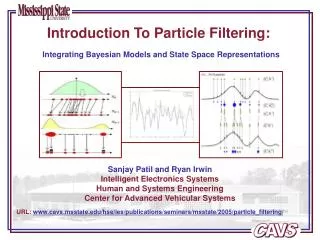
Applications of Particle Filters Particle filters have provided solutions to problems from many disciplines: • image processing and understanding • tracking complex objects (e.g. people) in video sequences • robot navigation • tracking and identifying complex military targets (e.g. vehicle convoys)
Advantages of Particle Filters • Under general conditions, the particle filter estimate becomes asymptotically optimal as the number of particles goes to infinity. • Non-linear, non-Gaussian state update and observation equations can be used. • Multi-modal distributions are not a problem. • Particle filter solutions to inference problems are often easy to formulate.
Disadvantages of Particle Filters • Naïve formulations of problems usually result in significant computation times. • It is hard to tell if you have enough particles. • The best importance distribution and/or resampling methods may be very problem specific.