Download
1 / 89
1k likes | 1.11k Views
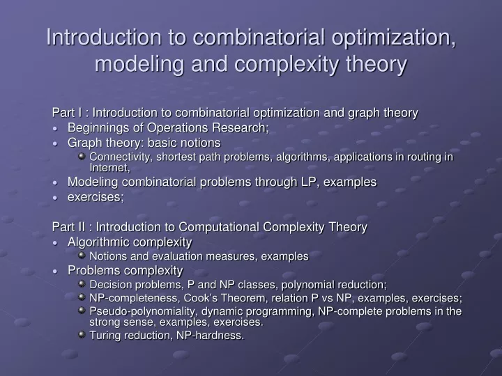
Introduction to combinatorial optimization, modeling and complexity theory. Part I : Introduction to combinatorial optimization and graph theory Beginnings of Operations Research; Graph theory: basic notions

E N D
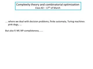
Introduction to combinatorial optimization, modeling and complexity theory Part I : Introduction to combinatorial optimization and graph theory • Beginnings of Operations Research; • Graph theory: basic notions • Connectivity, shortest path problems, algorithms, applications in routing in Internet, • Modeling combinatorial problems through LP, examples • exercises; Part II : Introduction to Computational Complexity Theory • Algorithmic complexity • Notions and evaluation measures, examples • Problems complexity • Decision problems, P and NP classes, polynomial reduction; • NP-completeness, Cook’s Theorem, relation P vs NP, examples, exercises; • Pseudo-polynomiality, dynamic programming, NP-complete problems in the strong sense, examples, exercises. • Turing reduction, NP-hardness.
History… • Léonard EULER: 1707-1783 • Seven Bridges of Königsberg • Charles BABBAGE: 1791-1871(Ada LOVELACE : 1815-1852) • Design of computers: Babbage sought a method by which mathematical tables could be calculated mechanically, removing the high rate of human error. • Alan TURING: 1912-1954 • The Turing machine • Decrypting the Enigma code (Combinatorial), • COLOSSUS: one of the first computers
History… • Léonid KANTOROVITCH : 1912- 1986 • a pioneer of linear programming… transport program, • Nobel price in economics (1975) • Georges Bernard DANTZIG : 1914- 2005 • Linear programming • Jeff HAWKINS : 1957 • Inventor of personnel-assistant (Palm Pilot)
History… • Paul ERDOS and Alfred RENYI • Albert-Lazlo BARABASI, Claude BERGE, Ken APPEL and Wolfgang HAKEN, • Jack EDMONS, Bernard Roy, Paul ROBERTSON et Neil SEYMOUR, Robert TARJAN
Some problems of Operations Research • Discrete combinatorial problems • Travelling salesman problem, • Minimum spanning tree • Continuous combinatorial problems • Linear programming, • Random problems • Queuing theory • Equipment replacement • Competitive situations • Game theory
Discrete combinatorial problemsTravelling salesman problem TSP. Given a set of n cities and a pairwise distance function d(u, v), is there a tour of length D? All 13,509 cities in US with a population of at least 500Reference: http://www.tsp.gatech.edu
Discrete combinatorial problemsTravelling salesman problem TSP. Given a set of n cities and a pairwise distance function d(u, v), is there a tour of length D? Optimal TSP tour Reference: http://www.tsp.gatech.edu
Continuous combinatorial problemsLinear programming Example. Suppose that a farmer has a piece of farm land, say A square kilometers large, to be planted with either wheat or cereals or some combination of the two. The farmer has a limited permissible amount F of fertilizer and P of insecticide which can be used, each of which is required in different amounts per unit area for wheat (F1, P1) and cereals (F2, P2). Let S1 be the selling price of wheat, and S2 the price of cereals. If we denote the area planted with wheat and cereals by x1 and x2 respectively, then the optimal number of square kilometers to plant with wheat vs cereals can be expressed as a linear programming problem: maximize (maximize the revenue) subject to: limit on total area) (limit on fertilizer) (limit on insecticide) (cannot plant a negative area)
Random problems • Queuing theory • applications to (internet) network congestion; • ordering the take-off of aircraft. • Equipment replacement • Deciding the replacement date for equipments with given failure probability.
Why using graphs? Seven bridges of Königsberg Given the above graph, is it possible to construct a path (or a cycle, i.e. a path starting and ending on the same vertex) which visits each edge exactly once?
Basic definitions • Directed Graphs • Non-oriented graphs • walks, cycles, paths, circuits • elementary • simple • Eulerian • Hamiltonian, • Stable, coloring, clique…
Basic definitions • A directed graph or digraph is a pair G= (X, U) of: • a set X, whose elements are called vertices or nodes, • a set U of ordered pairs of vertices, called arcs, directed edges, or arrows. • It differs from an ordinary, or undirected graph in that the latter one is defined in terms of edges, which are unordered pairs of vertices. • A valuated graph is G = (X, U, v) where (X, U) is a graph and v an application from U to R (real numbers). • Successors, predecessors, vertex degrees…
Basic definitions • A walk is an alternating sequence of vertices and edges, beginning and ending with a vertex, where each vertex is incident to both the edge that precedes it and the edge that follows it in the sequence, and where the vertices that precede and follow an edge are the end vertices of that edge. A walk is closed if its first and last vertices are the same (called a cycle), and open if they are different (called a path). • The lengthl of a walk is the number of edges that it uses. • A directed path is when edges are “has the same orientation” • A directed cycle: without the arrows, it is just a cycle. • A path is simple (resp. elementary), meaning that no vertices (resp. no edges) are repeated. • A graph is acyclic if it contains no cycles; • A path or cycle is Hamiltonian (resp. Eulerian) if it uses all vertices (resp. edges) exactly once.
Associated graphs • Partial Graph • Sub-graph • Complementary graph
Associated graphs • Transitive closure
Connectivity • Simple Connectivity: connected component • Strong Connectivity: strong connected component • Reduced Graph:
Connectivity and strong connectivity relations • An equivalence relation is a binary relation on a set that specifies how to split up (i.e. partition) the set into subsets such that every element of the larger set is in exactly one of the subsets. • reflexive, symmetric and transitive. • equivalence class ofx in E , denoted R(x), is given by: R(x)={y: xRy}. • What can-we say about connectivity and strong connectivity relations?
Particular Graphs • Forest is a graph without cycle • Tree is a connected graph without cycle
Particular Graphs • In graph theory, an arborescence is a directed graph in which, for a vertex v called the root and any other vertex u, there is exactly one directed path from v to u. A bipartite graph is a graph whose vertices can be divided into two disjoint sets U and V such that every edge connects a vertex in U to one in V;
Particular Graphs • In graph theory, a planar graph is a graph which can be embedded in the plane, i.e., it can be drawn on the plane in such a way that its edges intersect only at their endpoints. Graph of 3 entreprises () Complete Graph of 5 vertices ()
Basic definitions • An independent set or stable set is a set of vertices in a graph no two of which are adjacent. The size of an independent set is the number of vertices it contains (a(G)). • A maximal independent set is an independent set such that adding any other node to the set forces the set to contain an edge. • A clique in an undirected graph G, is a set of vertices V, such that for every two vertices in V, there exists an edge connecting the two. A clique in a graph G gives corresponds to a stable in its complementary graph and vice-versa.
Basic definitions • Some graph G is called c-chromatic if its vertices can be colored with c colors such that no two adjacent vertices have the same color. Similarly, an edge coloring assigns a color to each edge so that no two adjacent edges share the same color. Conjecture of 4 colors (1875 Pertersen) : “all planar graphs are -chromatic”
Coding a graph • Adjacency Matrix
Coding a graph • Successor queue b and a Exercise: Write an algorithm which allows the passage from the successor queue to the adjacency matrix.
Shortest path problems • Shortest path properties; • Polynomial algorithms for shortest path computation, examples and complexity: • Label correcting algorithms : Ford algorithm; • Label setting algorithms : Dijkstra algorithm, Bellman algorithm;
Shortest path problems • Some properties: • Lemma 1 • Any path extracted from a shortest path is also the shortest one. • Lemma 2 • A necessary and sufficient condition of existence of shortest paths is the absence of negative circuits. • Lemma 3 • let G be a graph without negative circuits and li the shortest path values from x0. A necessary and sufficient condition for that edge (xi, xj) is in a shortest path is : lj - li=vij.
Algorithm: (i) Initialization Poser l0 = 0 et li = + pour i > 0. (ii) Edges examination for each vertex xi, check all (xi,xj) from xi and substitute lj with li + vij when li +vij < lj. (iii) Stop Test Iterate (ii) until some lj is updated in (ii). FORD Algorithm An example
FORD Algorithm an example End of first iteration
FORD Algorithm an example End of second iteration
FORD Algorithm an example Last iteration
Validity et complexity of Ford algorithm Theorem 1: Ford agorithm computes values of the shortest path from x0 when the graph is without negative circuits. Theorem 2: The complexity of Ford algorithm is in O(nm) where n = |X| and m = |U|.
DIJKSTRA Algorithm Algorithm • set S ={x0}, l0 = 0, li =v0i, if (x0, xi )ÎU, and li=+, otherwise. (ii) while S X do: choose xiÎ X - S of li minimum. set S = S +{ xi }. For any xjÎ( X - S ), successor of xi, set: lj = min( li + vij, lj ).
DIJKSTRAAlgorithm an example End of the first iteration
DIJKSTRAAlgorithm an example End of the second iteration
DIJKSTRAAlgorithm an example End of the third iteration
DIJKSTRAAlgorithm an example End of the forth iteration
DIJKSTRAAlgorithm an example End of the last iteration
Validity and complexity of Dijkstra algorithm Lemma 4 Dijkstra algorithm is of complexity O(n2). Theorem 3 li obtained at the end of the algorithm are the shortest path values from x0.
Bellman algorithm Algorithm: (i) enumerate all vertex of the graph, set l0= 0. (ii) for j = 1 to n – 1 set : lj = min (lk + vkj ) over the set of predecessors xk of xj. Theorem 4: Bellman algorithm computes the shortest path values li from x0 in O(m).
Some path problems • The longest path computation problem; • The maximum probability path; • The maximum capacity path value; • Exercise : compute the shortest path among these of maximum capacity.
Exercise: The itinerary of Michel Strogoff (from ROSEAUX) Leaving from Moscow, Michel STROGOFF, courier of the tsar, was supposed to reach IRKUTSK. Before leaving, he had consulted a fortune teller who told him, amongst other things : "After KAZAN beware of the sky, in OMSK beware of the tartars, in TOMSK beware of the eyes, after TOMSK beware of water and, above all, always be careful of a large brown-haired person with black boots. " STROGOFF had therefore written on a map his "chances" of success for each route between two towns : these chances were represented by a number between 1 and 10 (measuring the number of chances of success out of 10). Ignoring probability calculation, he had therefore chosen his route by maximising the total sum of the chances. The numbers of the cities are: MOSCOW (1), KAZAN (2), PENZA(3), PERM (4), OUFA (5), TOBOLSK (6), NOVO-SAIMSK (7), TARA (8), OMSK (9), TOMSK (10), SEMIPALATINSK(11), IRKOUTSK (12). 1. Determine the route of Michel Strogoff. 2. What was the probability, with the assumption of the independence of the random variables, that Strogoff would succeed? 3. What would have been his route if he had known the principles of probability calculation?
Shortest path algorithms and applications to networks Routing protocols are implemented in a distributed way in IP networks.; What is routing …
What is routing? • The term routing corresponds to the mechanisms used by a host to transfer data to its destination by examining the information in the data. • Routing is a key element of level network of TCP/IP stack. It uses information stocked in routing tables in each node-router. • The routing table stores the routes (and in some cases, metrics associated with those routes) to particular network destinations. It is frequent that in a routing table we find only the information about the gateway number toward the destination and not the entirely route.
Routing Protocols in Internet Two main groups: – Distance-Vector protocols: RIP, IGRP, BGP. – Link-State protocols: OSPF, IS-IS
Distance-Vector routing protocols A variant of Bellman-Ford algorithm: boolean Bellman_Ford (G, s) initialization (G, s) // all weights are set to + except 0 for the origin node (0). for i=1 to Number_of_nodes -1 do: for any edge (u, v) do: wx := weight(u) + weight(edge(u, v)); if wx <weight(v) then pred(v) := u; weight(v) := wx; for any edge (u, v) do: if weight(u) + weight(edge(u, v)) < weight(v) then return false; return true.
Routing Information Protocol (RIP)(RFC 2453) Let D(i,j) represent the metric of the best route from entity i to entity j. It should be defined for every pair of entities. d(i,j) represents the costs of the individual steps. Formally, let d(i,j) represent the cost of going directly from entity i to entity j. It is infinite if i and j are not immediate neighbors. Since costs are additive, it is easy to show that the best metric must be described by: D(i,i) = 0, all i D(i,j) = mink [d(i,k) + D(k,j)], otherwise and that the best routes start by going from i to those neighbors k for which d(i,k) + D(k,j) has the minimum value.
Implementing RIP The Routing Information Protocol is a dynamic routing protocol used in local and wide area networks. As such it is classified as an interior gateway protocol (IGP) using the distance-vector routing algorithm. Each router keeps a distance table for all destinations in the network. This table stores all shortest distance to any destination and the next neighbor to reach each of them according to the distance. Periodically, each router announces its distance table to its direct neighbors; Any time some update is announced from a neighbor, do: compute the new distance D’; if D’ < D keep the new value and the neighbor announcing it; The update procedure is in origine of some limitations of the protocol…