Download
1 / 2
20 likes | 124 Views
Use Quality-Controlled PVT data to set up an EoS model of the reservoir. Ensure that gas Z-factors and C7+ content of the gas are matched accurately. Check the predicted depletion recoveries agree with CVD results.

E N D
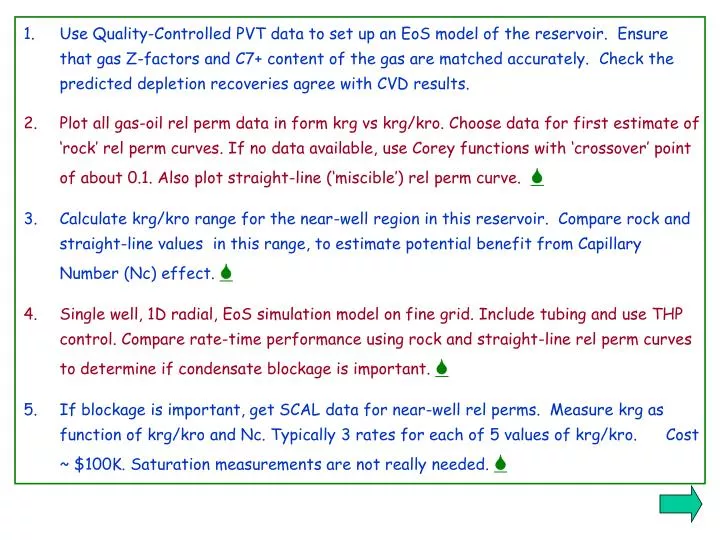
Use Quality-Controlled PVT data to set up an EoS model of the reservoir. Ensure that gas Z-factors and C7+ content of the gas are matched accurately. Check the predicted depletion recoveries agree with CVD results. • Plot all gas-oil rel perm data in form krg vs krg/kro. Choose data for first estimate of ‘rock’ rel perm curves. If no data available, use Corey functions with ‘crossover’ point of about 0.1. Also plot straight-line (‘miscible’) rel perm curve. • Calculate krg/kro range for the near-well region in this reservoir. Compare rock and straight-line values in this range, to estimate potential benefit from Capillary Number (Nc) effect. • Single well, 1D radial, EoS simulation model on fine grid. Include tubing and use THP control. Compare rate-time performance using rock and straight-line rel perm curves to determine if condensate blockage is important. • If blockage is important, get SCAL data for near-well rel perms. Measure krg as function of krg/kro and Nc. Typically 3 rates for each of 5 values of krg/kro. Cost ~ $100K. Saturation measurements are not really needed.
Set up fine grid single well model. Include cell-to-cell calculation of Nc effects. When using the E300 model for Nc effects, check that the behavior of krg versus Nc at fixed krg/kro matches experimental data. (If high-rate rel perm data are not available, use the Fevang-Whitson correlation with a = 4000, n=0.7), • Set up a coarse grid, single well model using the Generalized Pseudopressure Model (GPP in Eclipse). Include the Nc effect. Compare results with the fine grid single well model - they should agree, though for lean condensates it may be necessary to use smaller cells in the coarse grid. • Full field model using coarse grid and GPP model with Nc effects. In principle this calculation can use a black oil model with a table of IFT versus pressure, but this is not possible at present with Eclipse, so that a compositional model must be run. A large number of components is not needed – 5 or 6 should be sufficient.