Download

1 / 31
320 likes | 474 Views
Markov Models. Markov Chain. A sequence of states: X 1 , X 2 , X 3 , … Usually over time The transition from X t-1 to X t depends only on X t-1 (Markov Property). A Bayesian network that forms a chain The transition probabilities are the same for any t ( stationary process). X1. X2.

E N D
Markov Chain • A sequence of states: X1, X2, X3, … • Usually over time • The transition from Xt-1 to Xt depends only on Xt-1 (Markov Property). • A Bayesian network that forms a chain • The transition probabilities are the same for any t (stationary process) X1 X2 X3 X4
Courtsey of Michael Littman Example: Gambler’s Ruin • Specification: • Gambler has 3 dollars. • Win a dollar with prob. 1/3. • Lose a dollar with prob. 2/3. • Fail: no dollars. • Succeed: Have 5 dollars. • States: the amount of money • 0, 1, 2, 3, 4, 5 • Transition Probabilities
Example: Bi-gram Language Modeling • States: • Transition Probabilities:
Transition Probabilities • Suppose a state has N possible values • Xt=s1, Xt=s2,….., Xt=sN. • N2 Transition Probabilities • P(Xt=si|Xt-1=sj), 1≤ i, j ≤N • The transition probabilities can be represented as a NxN matrix or a directed graph. • Example: Gambler’s Ruin
What can Markov Chains Do? • Example: Gambler’s Ruin • The probability of a particular sequence • 3, 4, 3, 2, 3, 2, 1, 0 • The probability of success for the gambler • The average number of bets the gambler will make.
Working Backwards 325 287.5 B. Associate Prof.: 60 • Assistant • Prof.: 20 0.2 0.2 0.7 0.2 0.6 300 T. Tenured Prof.: 90 0.2 0.6 50 0.3 S. Out on the Street: 10 0.2 D. Dead: 0 0 0.8 1.0 Another question: What is the life expectancy of professors?
2/3 1 1 +1 1 1/3 Ruin Chain
+1 Gambling Time Chain 2/3 1 1 1/3
Kth-Order Markov Chain • What we have discussed so far is the first-order Markov Chain. • More generally, in kth-order Markov Chain, each state transition depends on previous k states. • What’s the size of transition probability matrix? X1 X2 X3 X4
Hidden Markov Model • In some Markov processes, we may not be able to observe the states directly.
A HMM is a quintuple (S, E, P, A, B ). S : {s1…sN } are the values for the hidden states E : {e1…eT } are the values for the observations P: probability distribution of the initial state A: transition probability matrix B: emission probability matrix Hidden Markov Model X1 Xt-1 Xt Xt+1 XT e1 et-1 et et+1 eT
Alternative Specification • If we define a special initial state, which does not emit anything, the probability distribution P becomes part of transition probability matrix.
Notations • Xt: A random variable denoting the state at time t. • xt: A particular value of Xt. Xt=si. • e1:t: an observation sequence from time 1 to t. • x1:t: a state sequence from time 1 to t.
Forward Probability • Forward Probability: P(Xt=si, e1:t) • Why compute forward probability? • Probability of observations: P(e1:t). • Prediction: P(Xt+1=si | e1:t)=?
Compute Forward Probability P(Xt=si, e1:t) = P(Xt=si, e1:t-1, et) = Xt-1=Sj P(Xt-1=sj, Xt=si, e1:t-1, et) = Xt-1=Sj P(et|Xt=si, Xt-1=sj, e1:t-1) P(Xt=si, Xt-1=sj, e1:t-1) = Xt-1=Sj P(et|Xt=si) P(Xt=si|Xt-1=sj, e1:t-1) P(Xt-1=sj, e1:t-1) = Xt-1=Sj P(et|Xt=si) P(Xt=si|Xt-1=sj) P(Xt-1=sj, e1:t-1) Same form. Use recursion
Compute Forward Probability (continued) αi(t) = P(Xt=si, e1:t) = Xt-1=Sj P(Xt=si|Xt-1=sj) P(et|Xt=si) αj(t-1) = j aij bietαj(t-1) where aij is an entry in the transition matrix biet is an entry in the emission matrix
Inferences with HMM • Decoding: argmaxx1:t P(x1:t|e1:t) • Given an observation sequence, compute the most likely hidden state sequence. • Learning: argmax P(e1:t) where =(P, A, B ) are parameters of the HMM • Given an observation sequence, find out which transition probability and emission probability table assigns the highest probability to the observations. • Unsupervised learning
Viterbi Algorithm • Compute argmaxx1:t P(x1:t|e1:t) • Since P(x1:t|e1:t) = P(x1:t, e1:t)/P(e1:t), • and P(e1:t) remains constant when we consider different x1:t • argmaxx1:t P(x1:t|e1:t)= argmaxx1:t P(x1:t, e1:t) • Since the Markov chain is a Bayes Net, • P(x1:t, e1:t)=P(x0) i=1,t P(xi|xi-1) P(ei|xi) • Minimize – log P(x1:t, e1:t) =–logP(x0) +i=1,t(–log P(xi|xi-1) –log P(ei|xi))
Viterbi Algorithm • Given a HMM (S, E, P, A, B ) and observations o1:t, construct a graph that consists 1+tN nodes: • One initial node • N node at time i. The jth node at time i represent Xi=sj. • The link between the nodes Xi-1=sj and Xi=sk is associated with the length –log(P(Xi=sk| Xi-1=sj)P(ei|Xi=sk))
The total length of a path is -logP(x1:t,e1:t) • The problem of finding argmaxx1:t P(x1:t|e1:t) becomes that of finding the shortest path from x0=s0 to one of the nodes xt=st.
Baum-Welch Algorithm • The previous two kinds of computation needs parameters =(P, A, B ). Where do the probabilities come from? • Relative frequency? • But the states are not observable! • Solution: Baum-Welch Algorithm • Unsupervised learning from observations • Find argmax P(e1:t)
Baum-Welch Algorithm • Start with an initial set of parameters 0 • Possibly arbitrary • Compute pseudo counts • How many times the transition from Xi-i=sj to Xi=sk occurred? • Use the pseudo counts to obtain another (better) set of parameters 1 • Iterate until P1(e1:t) is not bigger than P(e1:t) • A special case of EM (Expectation-Maximization)
Xt=si Xt+1=sj Pseudo Counts • Given the observation sequence e1:T, • the pseudo count of the state si at time t is the probability P(Xt=si|e1:T) • the pseudo counts of the link from Xt=si to Xt+1=sj is the probability P(Xt=si,Xt+1=sj|e1:T)
Update HMM Parameters • count(i): the total pseudo count of state si. • count(i,j): the total pseudo count of transition from si to sj. • Add P(Xt=si,Xt+1=sj|e1:T) to count(i,j) • Add P(Xt=si|e1:T) to count(i) • Add P(Xt=si|e1:T) to count(i,et) • Updated aij= count(i,j)/count(i); • Updated bjet=count(j,et)/count(j)
P(Xt=si,Xt+1=sj|e1:T) = P(Xt=si,Xt+1=sj, e1:t, et+1, et+2:T)/ P(e1:T) = P(Xt=si, e1:t)P(Xt+1=sj|Xt=si)P(et+1|Xt+1=sj) P(et+2:T|Xt+1=sj)/P(e1:T) = P(Xt=si, e1:t) aijbjet+1P(et+2:T|Xt+1=sj)/P(e1:T) = i(t) aij bjetβj(t+1)/P(e1:T)
Xt=si Xt+1=sj bj(t+1) ai(t) aijbjet t-1 t t+1 t+2
P(Xt=si|e1:T) =P(Xt=si, e1:t, et+1:T)/P(e1:T) =P(et+1:T| Xt=si, e1:t)P(Xt=si, e1:t)/P(e1:T) = P(et+1:T| Xt=si)P(Xt=si|e1:t)P(e1:t)/P(e1:T) = i(t) βi(t)/P(et+1:T|e1:t)