Download
1 / 28
350 likes | 656 Views
Comparing Genetic Algorithm and Guided Local Search Methods. Mehrdad Nojoumian & Divya Nair. Contents. Problem Clarification & Motivation Definition and Related Work Genetic Algorithms (GA) Guided Local Search (GLS) Experimental Results Conclusion & Future Work.

E N D
Comparing Genetic Algorithm and Guided Local Search Methods Mehrdad Nojoumian & Divya Nair David R. Cheriton School of Computer Science
Contents • Problem Clarification & Motivation • Definition and Related Work • Genetic Algorithms (GA) • Guided Local Search (GLS) • Experimental Results • Conclusion & Future Work
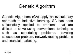
Problem Definition & Motivation • Problem: • Selecting the best strategy in order to solve various TSP instances • Many engineering problems can be mapped to the Travelling Salesman Problem • Motivation: • Compare two major AI approaches by the evaluation of their performance on TSPs • Genetic Algorithm (GA) • Guided Local Search (GLS) • Scrutinize behaviours of these techniques on the solution space
Y TSP instance: 48 capitals of the US X Definition and Related Work • Travelling Salesman Problem • Given a set of cities: represented as points in the plane with X & Y co-ordinates • The goal is to find the shortest tour that visits each city exactly once • It is an NP-complete problem • Related Work • Various GA implementations for TSP instances • Comparing various search strategy (not GA & GLS) • Hybrid approaches which combine GA and GLS
Sn Si S0 Local Search: HC, SA, TS, etc Global Max Local Max • Iterative process • Generate s0 • While (¬stopping condition) • Generate Neighbours N (si) • Evaluate N (si) • Si+1 = Select-Next N (si) • Return sn Exploitation Exploration
S4,0 S1,0 S3,0 S2,0 Population-Based: Genetic Algorithms Global Max Local Max • Iterative process • Generate p0 • While (¬stopping condition) • pm = Mutate(pi) • pc = Crossover(pm) • Pi+1 = Select(pc) • Return s* X Exploitation X Candidates for the next Generation Exploration
TSP Solution Space 500 ! = 1220136825991110068701238785423046926253574342803192842192413588385845373 1538819976054964475022032818630136164771482035841633787220781772004807852 0515932928547790757193933060377296085908627042917454788242491272634430567 0173270769461062802310452644218878789465754777149863494367781037644274033 8273653974713864778784954384895955375379904232410612713269843277457155463 0997720278101456108118837370953101635632443298702956389662891165897476957 2087926928871281780070265174507768410719624390394322536422605234945850129 9185715012487069615681416253590566934238130088562492468915641267756544818 8650659384795177536089400574523894033579847636394490531306232374906644504 8824665075946735862074637925184200459369692981022263971952597190945217823 3317569345815085523328207628200234026269078983424517120062077146409794561 1612762914595123722991334016955236385094288559201872743379517301458635757 0828355780158735432768888680120399882384702151467605445407663535984174430 4801289383138968816394874696588175045069263653381750554781286400000000000 0000000000000000000000000000000000000000000000000000000000000000000000000 0000000000000000000000000000000000000000
Genetic Algorithms (GA) Mutation 1 7 5 3 2 4 6 5 6 3 4 2 1 7 Generating Random Solutions Chromosomes 1 3 5 7 2 4 6 5 1 3 4 2 6 7 Combining Crossover 1 3 5 4 2 6 7 5 1 37 2 4 6 New Population 1 7 5 3 2 4 6 = 25 1 3 5 4 2 6 7 = 20 Offspring 1 7 5 3 2 4 6 5 6 3 4 2 1 7 1 3 5 4 2 6 7 5 1 3 7 2 4 6 Population 1 7 5 3 2 4 6 = 25 5 6 3 4 2 1 7 = 35 1 3 5 4 2 6 7 = 20 5 1 3 7 2 4 6 = 40 Evaluating Selecting
10 1 2 20 15 16 13 4 3 7 Fitness Function & Mutation • Fitness Function • Calculating the length of each path (chromosome) • Ch1: 1 2 3 4 1 = 10 + 13 + 7 + 16 = 46 • Ch2: 4 3 1 2 4 = 7 + 15 + 10 + 20 = 52 • … • Reciprocal Mutation • 1 2 3 4 5 6 7 8 9 ==> 1 2 6 4 5 3 7 8 9 • Inversion Mutation • 1 2 3 4 5 6 7 8 9 ==> 1 2 6 5 4 3 7 8 9
Crossover • Partially-Mapped Crossover • Pick crossover points A and B randomly and copy the cities between A and B from P1 into the child • For parts of the child's array outside the range [A,B], copy only those cities from P2 which haven't already been taken from P1 • Fill in the gaps with cities that have not yet been taken
Crossover (Cont.) • Order Crossover • Choose points A and B and copy that range from P1 to the child • Fill in the remaining indices with the unused cities in the order that they appear in P2
Selection • Rank Selection • Sort the population by their Fitness values • Each individual is assigned a Rank: R = 1for the best individual and so on • Then, the probability of being selected is P Rank : (0.5) 1 = 0.5 , (0.5) 2 = 0.25 , etc • Tournament Selection • Pick a handful of N individuals from the population at random (e.g. N = 20) • With a fixed probability: P (e.g. P = 1) choose the one with the highest fitness • Choose the second best individual with probability P * ( 1 - P ) • Choose the third best individual with probability P * ( ( 1 - P ) ^ 2 ) and so on
Local Search • Basic Idea Behind Local Search • Basic Idea: Perform an iterative improvement • Keep a single current state (rather than multiple paths) • Try to improve it • Move iteratively to neighbours of the current state • Do not retain search path • Constant space, often rather fast, but incomplete • What is a neighbour? • Neighbourhood has to be defined application-dependent
4 1 2 9 6 7 8 3 5 • A move operator • 2-opt? • Take a sub-tour and reverse it 9 1 4 2 7 3 5 6 8 9 reverse
4 1 2 9 6 7 8 3 5 • A move operator • 2-opt? • Take a sub-tour and reverse it 9 1 4 2 7 3 5 6 8 9 9 1 6 5 3 7 2 4 8 9
Guided Local Search (GLS) Goals: -To escape local minima -Introduce memory in search process -Rationally distribute search efforts GLS augments the cost function to include a set of penalty terms and passes the new modification to LS. LS is limited by the penalty terms and conducts search on promising regions of the search space. Each time LS gets caught in local minimum, the penalties are modified and LS is called again for the new modified cost function GLS penalizes solutions which contains specific defined features
Solution Features • A solution feature projects a specific property based on the major constraint expressed by the problem. For TSP, the solution features are edges between cities • A set of features can be defined by considering all possible edges that may appear in a tour with feature costs given by edge lengths. • For each feature, feature cost and penalty are defined. • A feature, fi is expressed using an indicator function as: Ii (s) = 1, solution s has property i, s Є S , S=set of all feasible solutions = 0, otherwise • In TSP problem, the indicator functions express the edges currently included in the candidate tour • The indicator functions are incorporated in the cost function to yield the augmented cost function
GLS Specifics As soon as the local minimum occurs during local search: • The penalties are modified and the cost function is upgraded to a new augmented cost function based on the following equation: h (s) = g (s) + λ . pi. Ii(s) g (s)-objective function M - is total set of features defined over solutions, λ - the regularization parameter pi - the penalty associated with feature, i. • The penalty vector is defined as: P = (p1, …, pM) • And the feature costs are defined by a cost vector: C = (c1, …, cM) • The penalty parameters are increased by 1 for all the features for which the following utility expression is the maximum:
Fast Local Search (FLS) • For speeding up local search • Through reduced neighborhood (sub-neighborhoods) • Method: • GLS + FLS : associate solution features to sub-neighborhoods • Associate activation bit to problem features • Procedure: • Initially all sub-neighborhoods active (bits to 1) • FLS called to reach first local minima • During modification action, only the associated sub-neighborhoods bits of penalized features are set to 1
Experimental Results 1. Comparison of GLS-FLS-2opt with GLS-greedy LS on s-TSP 2. Comparison of GLS-FLS-2opt with GA on s-TSP 3. Comparison of GLS-FLS-2opt with Branch and Bound on s-TSP GLS-FLS-2opt with GLS-greedy LS:
Comparison of GLS-FLS-2opt with GA • Mean Excess % • Mean CPU Time
Conclusion • GLS – GLS solver developed in C++ • GA – Java • Branch and Bound- Volgenant BB technique (Pascal) • The GLS-FLS strategy on the s-TSP instances yields the most promising performance in terms of near-optimality and mean CPU time • GA results are comparable to GLS-FLS results on the same s-TSP instances and it is also possible for the GA methods to generate near optimal solutions with a little compromise in CPU time (by increasing the number of iterations). • BB method generates the optimal solutions similar to GLS-FLS and the mean CPU time is better when compared to our GA approach and , the BB method can guarantee a lower bound for the given s-TSP instance, but works for only a maximum of 100 cities