Download
1 / 1
10 likes | 99 Views
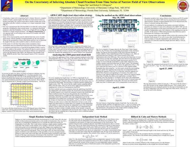
On the Uncertainty of Inferring Absolute Cloud Fraction From Time Series of Narrow Field of View Observations Yingtao Ma a and Robert G. Ellingson b a Department of Meteorology, University of Maryland, College Park, MD 20742

E N D
On the Uncertainty of Inferring Absolute Cloud Fraction From Time Series of Narrow Field of View Observations Yingtao Ma aand Robert G. Ellingson b aDepartment of Meteorology, University of Maryland, College Park, MD 20742 bDepartment of Meteorology, Florida State University, Tallahassee, FL 32306 0.8 0.7 q q q q 0.6 ARM-CART single-tract observation strategy To achieve our objective of testing the various PCLS models, we need to obtain cloud field properties such as the absolute cloud fraction (N), horizontal size and vertical thickness of clouds. At the ARM CART site, we have to rely on time sequences of vertically looking instruments to obtain the domain averaged value of these parameters. The question is, how well does the time averaged value represents the domain averaged value? Assuming the frozen turbulence approximation, the ARM sampling strategy can be seen as sampling the cloud field along a single transect line as shown below. Using the method on the ARM cloud observations May 30, 1999 • Abstract • Clouds play a major role in regulating Earth’s climate. However, computer models of Earth’s climate neglect the effects of cloud vertical extent in a broken cloud field. The vertical extent allows clouds to shade more of the atmosphere and allow radiative exchange over a larger temperature range (Fig. 1). • One way to parameterize this 3D cloud effect is to relate the various cloud properties, including the cloud vertical extent, to a statistical cloud field parameter called the Probability of Clear Line of Sight (PCLS) (see Fig. 2) and then to a simple integral parameter - the effective-cloud-fraction. In our ongoing study, we are trying to test various PCLS models with ARM cloud observations. • Many of the cloud properties must be inferred from time series of zenith observations, whereas spatially averaged quantities are the ones desired. What are the uncertainties of these observations and how can we determine the length of the time series needed to achieve a desired accuracy? • In this poster, we will show that under certain assumptions, these uncertainties may be evaluated from the given time series of observations. • A simulated cloud field from a Cloud Resolving Model (CRM) is used to show the validity of the method. The method will also be used to estimate the absolute cloud fraction from several narrow field of view instruments, such as the Micropulse Lidar (MPL), the Millimeter-Wavelength Cloud Radar (MMCR) and the Video Time-Lapsed Camera (VTLC, around its zenith). • Conclusions • Quantities needed to test various effective cloud fraction and PCLS models are measured at the ARM CART sites by assuming the frozen turbulence approximation. Domain averaged quantities have to be inferred from time series of vertically-looking observations. • Several methods of evaluating the uncertainties associated with these quantities are studied. If a time series obtained at the ARM CART site can be a good representative of the target cloud field and if it covers sufficient number of independent scales, the evaluation of the sampling error may be possible. In this poster a CRM model generated cloud field was used to demonstrate the usefulness of the methods. • In our ongoing studies, these methods will be used on the extraction of the absolute cloud amount, N, as well as some other cloud field properties. Some examples of using the independent scale method (Eq. 1) on the estimation of N from the cloud base height data from ARSCL VAP are shown here. 0.5 0.4 0.3 0.2 b =0.5 b =1.0 0.1 b =2.0 0 0 10 20 30 40 50 60 70 80 90 June 8, 1999 This cloud field is made from Bjorn Stevens' simulation of boundary layer clouds. The original Cloud Resolving Model (CRM) field has a domain size of 6.8 km2 with 0.1 km and 0.04 km horizontal and vertical grid-spacing and 0.57 cloud fraction. The above field is a mosaic of 8 original cloud fields. The red dotted line simulates the sampling tract of a narrow field of view instrument. Fig. 5a is a sequence of images taken by the Time Lapse Video Camera (TLCV). Fig. 5b shows the corresponding measurement of the cloud base height. The data are from the product of the Active Remote Sensing of Clouds (ARSCL) Value Added Product(VAP) (Clouthiaux, et.al., 2001). It represents their best-estimate of the vertical location of the cloud hydrometeors above the ARM sites. The x-axis gives the Julian time of every observation in seconds since midnight. The time interval of the observations is 40 seconds. From the cloud base height measurement and the TLCV images we can see that the cloud field is a quite stable single-layer clear weather cumulus cloud field which lasts for about 3 hours. The estimated absolute cloud amount N=0.5. Fig. 5c shows the application of Eq. 1. The curve represents the relative error as a function of line segment length. Remember that when using Eq. 1 we first need to divide the total sampling line into smaller line segments and assume they are independent before applying the equation. From Fig. 5c we find that, when the segments are shorter than 20 points (corresponding to 14 minutes), the relative error increases as the segment length become longer, whereas for segment lengths longer than 20 points, the relative error approaches a constant. This is expected, since the 20 points or 14 minutes can be seen as the independent scale of this cloud field. That is, two observations made 14 minutes apart can be considered as independent of each other. Of course two observations made more than 14 minutes apart will be independent of each other too. Analyzing the CRM generated cloud field Fig. 4 shows the application of four variance estimation methods on the CRM cloud field above (Fig. 3). The y-axis is the relative error (SN/N); x-axis is the length of the sampling line in pixels. The curve is obtained as follows: Introduction Fig. 7a shows the estimated cloud amount (N=0.18), which is much less than on April 2 (N=0.87 ). Figs. 7b, c show the relative error and application of Eq. 1. Figure 1 Vertically extended clouds projected lengths at angle q April 27, 1999 Figure 4 Plane parallel lengths Figure 5a To account for finite size effects of clouds on longwave radiation, one may define an effective-cloud-fraction(Ne). Ne is the plane-parallel cloud fraction that generates the same flux as the detailed models for a given broken cloud field after taking into account the effects of geometric shapes, size, spatial distribution and absolute amount (N) of clouds. These effects may be integrated into Ne through a single cloud field property – the PCLS. (1) For every sampling line length from 1 to 1200 at a step-length 20, we randomly do 30 simulated single-line measurements. This gives 30 estimates of the cloud amount N. Based on these 30 estimates of N, the relative error is calculated for that length. This procedure is repeated until the sampling line length reaches 1200. We can see that the simple random sampling method differs from the others. They all can be used to approximately predict the sampling error, at least for a homogeneous cloud field. The three methods need some assumption about the underlying cloud field. The independent scale method assumes the cloud field to be homogeneous; the HC method requires every cloud to be randomly located in the cloud field; the Matern method assumes the process that generates the cloud field is a stationary random process. In applying these methods we have to have some information about the cloud field, such as the independent scale for the independent scale method, the covariance[Cov(h)] for the Matern methods and the variance of cloud and clear intercepts(Slcld and Slclr) for the HC method. Without any other source to obtain this information we have to rely on the single-tract observations to evaluate them. For example, for the independent scale method, we need to determine the independent scale of the cloud field and the variance within the scale (the variance for every independent line segment). In order to obtain a reliable estimate of the variance, except the assumption that every independent sub-area has the same variance, one should also expect that the sampling line is long enough to cover a sufficient number of independent segments. PCLS for Random Cylindrical Clouds This day demonstrates a failure of using Eq. 1. We can see that the relative error (8b) increases as the segment length increases. This is mainly due to increasing cloud cover during the period. For this type of cloud field, we can not find a independent scale from our single-tract observations. Thus Eq. 1 can not be used in this situation. April 2, 1999 Figure 2 Figure 5b Figure 5c PCLS () b - Aspect Ratio - Height/Diameter (2) This day features a long lasting cumulus cloud field. Fig. 6a shows the cloud base height, and 6b is an application of Eq. 1. Fig. 6c is similar to Fig. 4, showing the relative error as a function of the sampling line length. The thin dashed line is the prediction of the simple random sampling method, which would underestimate the sampling error. Zenith Angle (Degrees) For a given absolute cloud fraction, N, PCLS(q) depends upon cloud shape, aspect ratio, spacing and horizontal distribution. Measurements of the angular variation of PCLS(q) allow tests of the various proposed models. (3) Hilliard & Cahn and Matern Methods Hilliard and Cahn (1961) (denoted as HC) and Matern (1986) also addressed the same problem. By assuming the sampling line is randomly located in the cloud field and every cloud is randomly dropped in the cloud field, HC gives the following formula to estimate the relative variance of N: Simple Random Sampling Suppose we want to estimate the absolute cloud amount by N=m/M, where M is the total number of observations (red points) and m is the number of cloud points. One way (not a good one) of evaluating the sampling error it to consider the observation points are independent of each other. This is equivalent to making a simple random sampling of the cloud field. The variance of the estimate of N is simply (1-N)*N/M. Of course the observation points are not independent of each other. Suppose the sampling rate is high enough and the horizontal size of the individual clouds is larger than the sampling interval (=time interval*wind speed). Then, on the small scale, the observation points maybe correlated to each other because of the possibility of several consequent points falling in a same cloud, and on the large scale, the points maybe correlated to each other because of the large scale dynamic environment of the cloud field. Usually the simple random sampling method will underestimated the measurement variance. Independent Scale Method An observation may be not independent of a near neighbor, but at some distance away two data points may be independent of each other. This directs us to another way of evaluating the uncertainties of single-tract measurements of the cloud amount. The method is based on the assumptions that the cloud field is homogeneous above a certain finite scale. That is, the whole cloud field may be considered as a mosaic of many pieces of sub-areas with finite scales and the same within-area variance. We call the maximum of these scales an independent scale. Pixels within the sub-area scale are correlated to each other, but beyond the scale, pixels are independent. If we make a measurement along a line that is several times longer than the independent scale, the line can be divided into several independent line segments.The estimate of the variance of N can be expressed as where lcld and lclr are the individual intercept lengths in the clouds and clear sky; M is the total number of intercepts. Matern’s method is based on the assumption that the cloud field is a realization of a random process. The variance of the domain mean estimated from a straight line is given as where Cov(h) is the covariance function of the isotropic process; h is the distance between two points chosen independently on the straight line with total length L. where Ni is the cloud fraction calculated within an independent segment; k is the number of segments; SN denotes the standard deviation of N. This is actually the standard method used to estimate the variance of the average of several independent random variables. Only here we consider the chains of observation points as the independent quantities but not the individual points. Figure 3 Figure 6c Figure 6a Figure 6b Figure 7c Figure 7a Figure 7b Figure 8a Figure 8b