Download
1 / 47
540 likes | 1.29k Views
Industrial Calculations For Transient Heat Conduction . P M V Subbarao Professor Mechanical Engineering Department IIT Delhi. Applications where rate/duration of heating/cooling is a Measure of Quality……. General Form of Fourier’s Equation . Cartesian coordinates:. Cylindrical coordinates:.

E N D
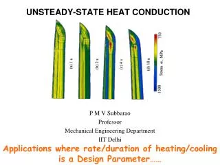
Industrial Calculations For Transient Heat Conduction P M V Subbarao Professor Mechanical Engineering Department IIT Delhi Applications where rate/duration of heating/cooling is a Measure of Quality……
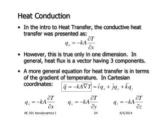
General Form of Fourier’s Equation Cartesian coordinates: Cylindrical coordinates: Spherical coordinates:
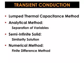
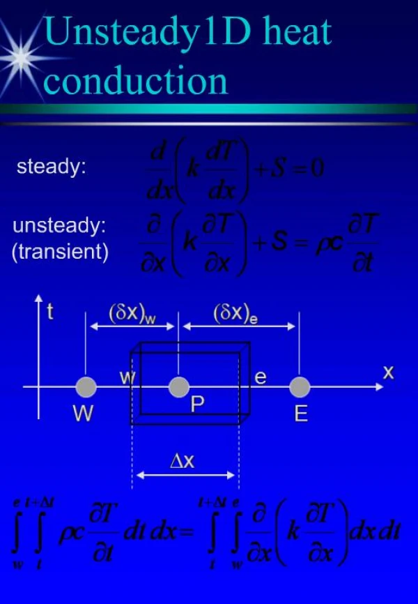
One-dimensional Transient Conduction : Finite Value of Biot Number • One-dimensional transient conduction refers to a case where the temperature varies temporally and in one spatial direction. • For example, temperature varies with x and time. • Three cases of 1-D conduction are commonly studied: conduction through a plate, in a cylinder, and in a sphere. • In all three cases, the surface of the solid is exposed to convection. • The exact analytical solutions to the three cases are very complicated. • Industry uses an approximate solution, obtained by using graphical tools. • The graphs allow you to find the centerline temperature at any given time, and the temperature at any location based on the centerline temperature.
One Dimensional Fourier’s Equations Constant thermal conductivity & No heat generation: Cartesian coordinates: Cylindrical coordinates: Spherical coordinates:
Primitive Variables & derived Variables Characteristic Space Dimension : L or ro Characterisitc Time Dimension : ? Characteristic Temperature Variables: Initial Temperature : T0 Far Field Fluid Temperature : T Characterisitc Medium Property : a
Extent of Solution Domain Highest Measure of Excess Temperature : q0 =|T0 -T| Instantaneous local Excess temperature: q =|T -T| Cartesian coordinates: Cylindrical coordinates: Spherical coordinates:
Nature of Solution Cartesian coordinates: Cylindrical coordinates: Spherical coordinates:
One Dimensional Transient Conduction Governing Differential Equation: Initial Condition: T(x,o)= T0 Boundary Conditions: T(L,t)=TsT
Non-dimensionalization of GDE Define a Non dimensional variable for the x-coordinate Define a Non dimensional variable for the temperature: Substitute Dimensionless variables into GDE:
Define thermal diffusivity: Define non dimensional variable for time : Fourier Number The Fourier number (Fo) or Fourier modulus, named after Joseph Fourier, is a dimensionless number that characterizes transient behavior of a system. Conceptually, it is the ratio of the heat conduction rate to the rate of thermal energy storage. It is defined as:
A Pure Dimensionless GDE Initial condition: q(h,0) = 1 Boundary conditions: q(1,z) = 0 At any time Temperature profile will be symmetric about x-axis. Solution in positive or negative direction of x is sufficient.
Simplified Problem 1 Initial condition: q(h,0) = 1 Boundary conditions: q(1,z) = 0 0 1 h
Heisler Parameters • Heisler divided the problem into two parts. • Part 1 : Instantaneous center line temperature. Variables are q0,,L, t, and a. • Part 2 : Spatial temperature distribution for a given center line temperature at any time. Variables are : qcenter,,x,L, and a. • Two different charts were developed. • Three parameters are needed to use each of these charts: • First Chart : • Normalized centerline temperature, • the Fourier Number, • and the Biot Number. • The definition for each parameter are listed below:
Second Chart : Frozen Time Parameter • Normalized local temperature, • Biot Number. • Spatial Location. • The definition for each parameter are listed below:
Internal Energy Lost by the Slab E0 is the Initial internal energy possessed by the slab by virtue of T0 After a time t, the slab has a temperature distribution, T(x,t): Let Qis the change in Initial internal energy of the slab during time t Define a non-dimensional change in energy: With
Multi-dimensional Transient Conduction Finite Cartesian Bodies: Finite Cylindrical Bodies:
Multi-dimensional Conduction • The analysis of multidimensional conduction is simplified by approximating the shapes as a combination of two or more semi-infinite or 1-D geometries. • For example, a short cylinder can be constructed by intersecting a 1-D plate with a 1-D cylinder. • Similarly, a rectangular box can be constructed by intersecting three 1-D plates, perpendicular to each other. • In such cases, the temperature at any location and time within the solid is simply the product of the solutions corresponding to the geometries used to construct the shape. • For example, in a rectangular box, T(x*,y*,z*,t) - the temperature at time t and location x*, y*, z* - is equal to the product of three 1-D solutions: T1(x*,t), T2(y*,t), and T3(z*,t).
Relationship between the Biot number and the temperature profile.
Systems with Negligible Surface Resistance • Homeotherm is an organism, such as a mammal or bird, having a body temperature that is constant and largely independent of the temperature of its surroundings.
Biot Number of Small Birds Bi Fur Thickness, cm
Biot Number of Big Birds Fur Thickness, cm
Very Large Characteristic Dimension The United States detonated an atomic bomb over Nagasaki on August 9, 1945. The bombings of Nagasaki and Hiroshima immediately killed between 100,000 and 200,000 people and the only instances nuclear weapons have been used in war.
The semi-infinite solid Governing Differential Equation: Boundary conditions x = 0 :T = Ts As x → ∞ :T → T0 Initial condition t = 0 :T = T0
Notice that there is no natural length-scale in the problem. Indeed, the only variables are T, x, t, and α.


![Chapter 3: Unsteady State [ Transient ] Heat Conduction](https://cdn1.slideserve.com/2468294/chapter-3-unsteady-state-transient-heat-conduction-dt.jpg)