Download
1 / 28
280 likes | 550 Views
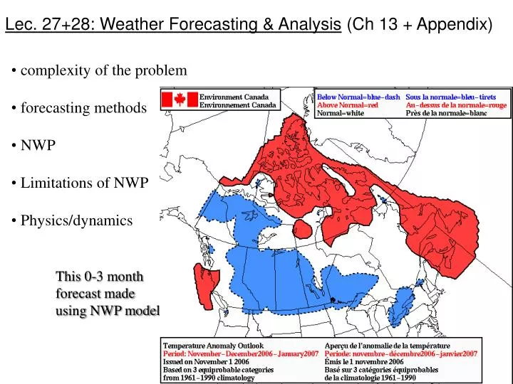
Lec. 27+28: Weather Forecasting & Analysis (Ch 13 + Appendix). complexity of the problem forecasting methods NWP Limitations of NWP Physics/dynamics. This 0-3 month forecast made using NWP models. Historical skill of this long-range dynamical forecast.

E N D
Lec. 27+28: Weather Forecasting & Analysis (Ch 13 + Appendix) • complexity of the problem • forecasting methods • NWP • Limitations of NWP • Physics/dynamics This 0-3 month forecast made using NWP models
Historical skill of this long-range dynamical forecast Modern NWP for the Normandy (D-day) landings based on data available at the time… http://www.ecmwf.int/research/era/dday/
This 3 month lead-time forecast made using statistical method
courtesy of Edward Hudson, Prairie & Arctic Aviation Weather Centre, Edmonton • taken 15 Nov., 2006
RAIN FELL FROM overcast skies and gale force winds drove large waves on to the beaches of Normandy as dawn broke on Monday June 5, 1944. To the Germans watching their defences, there was nothing to show that this was the moment the Allied Armies had planned to invade Europe. In fact, the operation had been put on hold because the bad weather had been forecast 24 hours before. Had it gone ahead in these conditions, the invasion would have been a catastrophic disaster. Nevertheless, the invasion had to occur on either the 5th, 6th or 7th of June to take advantage of the right conditions of moon and tide. Darkness was needed when the airborne troops went in, but moonlight once they were on the ground. Spring low tide was necessary to ensure extreme low sea level so that the landing craft could spot and avoid the thousands of mined obstacles that had been deployed on the beaches. If this narrow time slot was missed, the invasion would have to be delayed for two weeks. From “The Most Important Forecast in History,” by E. Brenstrum (N.Z. Meteorological Service). Published in New Zealand Geographic, pp11-16, Vol. 22, 1994,
Fluxes of longwave radiation (temperature-and composition- dependent) water/ice /vapour Cloud temperature pressure Boundary fluxes of heat and moisture (QH, QE) and momentum (frictional drag t ) on complex terrain vertical wind horizontal wind Fluxes of solar radiation (interact with clouds) variables inter-linked by consv. of mass, heat & momentum. Relations expressed as partial differential eqn’s winds on range of scales down to millimeters - cause advection, entrainment, etc.
Forecasting** methods Value of a given technique depends on “range” of the forecast. For now, focus on “weather” forecast… ie. range of up to a couple of weeks • Climatology:hard to beat for f/c ranges beyond about 10 days. • “The average.” eg., this afternoon’s weather in Edmonton will equal the average observed 1961-1990 for Nov. 15 in Edmonton • or, (eg.) this afternoon’s weather will be that associated with one of a set of “map types,” ie. previously observed on an afternoon having similar maps. Called an “analog method”... Ah! We’ve seen this… in 1901 … • or, forecast the anomaly associated with (eg.) Southern Oscillation Index • Persistence:hard to beat for f/c range of a few hours - eg. This afternoon’s weather same as this morning’s, except for influence of local processes (eg. solar heating) • Numerical Weather Prediction: hard to beat for f/c range out to about 10 days (esp. if supplemented by experienced human interpretation) ** “nowcasting” and “hindcasting”
“Causal” weather prediction (pre-computer age) • Detailed analysis of “initial state,” using hand-plotted weather maps & charts • Interpretation using rules and conceptual models (such as Polar Front theory, etc) having a physical basis, eg. • Atmospheric stability • air-sea interaction • local diurnal cycle - surface energy balance • Richardson’s pioneering hand-computation • science degree Cambridge 1903 • applied calculus to help Nat’l Peat Co. cut drains in peat • 1913 joined Meteorol. Off. (supervised an observatory) • ambulance driver, WW1 France • in off-duty time, embarked on test of his mathematical forecasting system… had taken with him to France observations for 7 a.m., 20 May 1910. • by 1916, wrote Weather Prediction by Arithmetic Finite Differences… published 1922 Lewis Fry Richardson (1881-1953)
Richardson divided a map of Europe into squares… for each he tabulated atmospheric pressure… armed with a slide rule and mathematical tables, he began the laborious task of 'forecasting' what was going to happen to the weather at 1 p.m. on his selected day… producing by hand a six-hour weather forecast which he could check against observations. For each square on his map, he applied his numerous equations, to calculate changes of pressure, wind and temperature… The six-hour forecast took him six weeks. And when he had finished, the forecast was horribly wrong. Images and quotation from P. Holper, Australian Broadcasting Corp., http://www.abc.net.au/science/slab/forecast/story.htm For an excerpt from Richardson’s book, see http://alumnus.caltech.edu/~zimm/weather.html
Numerical Weather Prediction • Based on the physics as expressed in equations… conservation of mass, momentum, energy + equations of state + (etc.) • set of coupled “partial differential equations” for U,V,W,T,Q… versus x,y,z,t (or more typically lat., long., pressure and time) • which can be solved numerically given “initial” and “boundary” conditions (eg. sea surface temperature + much more) • produces gridded fields of U,V,W,T,Q,… • to produce forecast numerical output supplemented by rules of thumb, statistical packages, subjective guidance
data acquisition • analysis phase • initialisation (t=0) • prediction phase (numerical integration) • post-processing phase Stages in NWP
The decision to postpone the invasion for 24 hours had been taken by Eisenhower and the Supreme Command at 0430 on Sunday June 4. It was not taken lightly, because so many ships were already converging on Normandy that the risk of detection was grave. Nor had the forecast which prompted the postponement been easily arrived at. Eisenhower's weather advice was provide by Group Captain Stagg, a forecaster seconded from the British Meteorological Office who was coordinating the advice of three forecasting teams: one from the Meteorological Office, one from the Admiralty and one from the United States Army Air Forces. The advice of these groups was often diametrically opposed. The American team used an analog method, comparing the current map with maps from the past, and were often over-optimistic. The Meteorological Office, aided by the brilliant Norwegian theoretician Sverre Petterssen, had a more dynamic approach, using wind and temperature observations from high altitude provide by the air force, and were closer to the mark. The decision to invade on Tuesday June 6, taken late on Sunday night and finally confirmed early Monday morning, was based on a forecast of a short period of improved weather caused by a strengthening ridge following the front that brought Monday's rain and strong winds. In the event, Monday's bad weather had already given the Allies a crucial advantage: it had put the Germans off guard. From New Zealand Geographic, pp11-16, Vol. 22, 1994
Data acquisition • regional or global? (depending on f/c range) • obs. coordinated by World Meteorol. Org. • 10K land obs stations, 7K ship obs, 300 buoys, weather satellites, 1K radiosondes twice daily + (still in research phase) sensors on scheduled commercial aircraft +… • “synoptic times” 0000 and 1200 UTC (GMT), but increasing amount of data comes in off the synoptic times… challenge to incorporate these Doppler wind sounders (acoustic & electromagnetic) Surface winds from satellite scatterometry
The traditional in-situ synoptic data… Fig. 13-3 Rawindsonde
Analysis Phase • quality control… criteria of physical acceptability (eg. no negative pressures) and plausibility relative to climate • interpolation onto a regular “grid” of points • numerical analysis: adjustment to form fields that are consistent with allowable physics (eg. winds must be such that air mass is conserved) and consistent with the numerical model being used (eg. initial data must not contain features the model is unable to resolve, eg. reduced winds in a small valley not “visible” in model’s terrain) • the “adjustment” blends the observations for time t0 with a 6 hour forecast valid for t0
Data on a grid (shown in 2-d), example of “interpolation”, and finite-difference representation of a gradient J+1 J TI-1, J TI+1, J TI, J J-1 Dx I-1 I I+1 n w e
Building an equation to express conservation of air mass on the grid rI , J rI-1 , J-1 Fz(z2) “flux” of air is a vector with components Fx,y,z [kg m-2 s-1] Wind components: U,V,W z2 Dz Fx(x1) Fx(x2) z1 Since flux is convective, Fz(z1) Dx x1 x2
rI , J rI-1 , J-1 … expresses the change IJin time t of the mass [kg] of air in box IJ. (Note: y is the face length along y) Fz(z2) z2 Dz Fx(x1) Fx(x2) z1 Thus we need to interpolate values of U and r on “control volume faces” Fz(z1) Dx x1 x2
Numerical integration (prediction phase) Governing equations have form (eg.) (term shown on r.h.s. is advection of heat along the x-axis). On re-arrangement one has a formula to advance the temperature at gridpoint (I,J,K) over time interval t (15 minutes, GEM global, Nov. 06) from time “n” to time “n+1” Repeat the process to go from time “n+1” to “n+2”… out to 12, 24, 36, 48 hours (or longer). End result: forecast fields of U,V,W,T,P, r, Q (humidity) on the grid
Post-processing phase • produce and distribute maps for mandatory levels, to convey model output to forecasters • Forecast products usually involve subjective human involvement. Forecaster compares models, knows which aspects of which models have proven reliable ALERT: Received the following bulletin at Mon Dec 02 08:04:08 UTC. MAIN WX DISCUSSION, UPPER LEVEL PATTERN WHILE OVER W CST THE L/W UPPER RIDGE WILL PERSIST, CONDITIONS WILL BE QUITE ACTIVE IN THE VAST CYCLONIC CIRCULATION COVERING ALMOST ENTIRE CANADA AND ARCTIC... HOWEVER DESPITE THIS HIGHLY CHANGING UPPER LEVEL PATTERN, MODELS ARE IN QUITE GOOD AGREEMENT FOR THE UPPER LEVEL PATTERN EVOLUTION NEXT 48 HRS. SINCE REGGEM HAS VERIFIED THE BEST PAST RUN AND IS VERY CONSISTENT, WE ACCEPT ITS SCENARIO. • may use rules of thumb and/or supplementary statistical algorithms to forecast weather elements, eg. tomorrow’s max or visibility for an airport
The “omega-block” (or “omega high”) • tends to persist • predictable weather • useful hint to forecaster Fig. 13-17
Weather in relation to Operation Uranus – Soviet encirclement of besieging German 6th Army at Stalingrad; 19 Nov., 1942 From Ch15 of A. Beevor’s “Stalingrad. The Fateful Siege: 1942-1943” “All through the night, Soviet sappers in white camouflage suits had been crawling forward in the snow, lifting anti-tank mines… One Soviet general said that the freezing white mist was `as thick as milk’… Front headquarters considered a further postponement, due to the bad visibility, but decided against it… `Once again, the Russians have made masterly use of the bad weather,’ wrote (General von) Richthofen During the afternoon of 19 November, the Soviet tanks advanced southwards in columns through the freezing mist… it was Butkov’s 1st Tank Corps which finally encountered the gravely weakened 48th Panzer Corps. The German tanks still suffered from electrical problems, and their narrow tracks slid around on the black ice. The fighting in the gathering dark was chaotic. The usual German advantages of tactical skill and coordination were entirely lost.”
Model Output Statistics (MOS) • Forecasting algorithm that employs an established (historical) statistical correlation between: • past observed values of weather variables (eg. visibilityV), and • corresponding forecast values of a set of “relevant” variables from NWP model (eg. local 500 mb height H500, wind speed and direction at 850 mb, U850, b850, etc.) • of form V = V (H500, U850, b850, ... ) • used predictively with machine forecasts to predict future weather • this partly “corrects” flaws in NWP model. But MOS correlations must be re-calculated (“re-trained”) for each revision of NWP model
Medium-range forecasting • Numerical forecast for ranges of order 3-15 days • not much skill beyond one week • increasingly common to perform “ensemble forecast” (multiple model runs starting from slightly different initial conditions that attempt to mimic possible errors in the initial data). Variability of the forecast amongst ensemble-members implies greater uncertainty Long-range seasonal anomaly forecasting • Statistical techniques presently the most important • where numerical models involved, must be coupled land-atmosphere-ocean • at present, low skill
Attributes of NWP models • domain & boundary conditions (eg. if global, no lateral boundaries) • spatial and temporal resolution • grid or spectral representation? • model “dynamics” (approximations in the equations, eg. hydrostatic?; choice of dependent variables, eg. velocity or vorticity?...) • model “physics” (which includes “parameterizations” of effects of unresolved scales of motion): • radiation as function of model’s diagnosed cloud and possibly other resolved properties such as humidity, CO2 concentration… • convection (deep & shallow), clouds (stratiform & cumuliform) & precip • surface exchange (momentum, heat, vapour, CO2…) based on surface state, analyzed or forecast • drag on unresolved terrain features trade-offs in speed vs. detail
Compromising limitations of numerical weather forecasting • extreme sensitivity to initial data (growth of initial errors) • data-sparse regions • inability to represent all scales of motion, from the planetary down to the scale of a cloud droplet • at present, grid-spacing order 10 km in horiz… thus for example no possibility to model cumulus… effects of cumulus must be “parametrized” (eg. diagnose cloud base and cloud top height from model’s temperature and humidity profiles: re-mix heat and vapour uniformly in that layer) • some processes entirely missing • others (eg. land-atmosphere exchange, drag on small hills) oversimplified/poorly represented
Forecast Assessment Quality --- Value skill accuracy • considered “skillful” if provides (in a statistical sense) greater accuracy than persistence or climatological forecasts • forecasting extremes: valuable when right, penalizing when wrong - forecasters reluctant to forecast extremes, more likely to be correct if f/c near-average conditions • types of f/c include qualitative (categorical), quantitative, probability f/c • many criteria exist for accuracy of f/c, eg. mean absolute error (MAE) average magnitude of difference between f/c and actuality