Download
1 / 32
320 likes | 444 Views
Central limit theorem - go to web applet. Correlation maps vs. regression maps. PNA is a time series of fluctuations in 500 mb heights PNA = 0.25 * [ Z(20N,160W) - Z(45N,165W) + Z(55N,115W) - Z(30N,85W) ]. index vs. time. PNA - Correlation map (r values of each point with index).

E N D
Correlation maps vs. regression maps PNA is a time series of fluctuations in 500 mb heights PNA = 0.25 * [ Z(20N,160W) - Z(45N,165W) + Z(55N,115W) - Z(30N,85W) ] index vs. time
PNA - Correlation map (r values of each point with index) PNA - Regression map (meters/std deviation of index) Correlation maps vs. regression maps PNA is a time series of fluctuations in 500 mb heights PNA = 0.25 * [ Z(20N,160W) - Z(45N,165W) + Z(55N,115W) - Z(30N,85W) ] Correlation maps put each point on ‘equal footing’ Regression maps show magnitude of typical variability
Empirical Orthogonal Functions (EOFs): An overview What are the dominant patterns of variabililty in time and space? Mathematical technique which decomposes your data matrix into spatial structures (EOFs) and associated amplitude time series (PCs) The EOFs and PCs are constructed to efficiently explain the maximum amount of variance in the data set. By construction, the EOFs are orthogonal to each other, as are the PCs. In general, the majority of the variance in a data set can be explained with just a few EOFs. Provide an ‘objective method’ for finding structure in a data set, but interpretation requires physical facts or intuition.
3 “Products” of Principle Component Analysis Singular Value Decomposition (SVD)X = USVT 1) Eigenvectors Some 2-D Data (X) 2) Eigenvalues 3) Principle Components Eigenanalysis XXT = C; CE = LE
Examples for Today 1) Eigenvectors – Variations explained in space (MAPS) Fake and Real Space-Time Data (X) 2) Eigenvalues - % of Variance explained (spectrum) 3) Principle Components Variations explained in the time (TIMESERIES)
Eigenvectors, Eigenvalues, PC’s • Eigenvectors explain variance in one dimension; Principle components explain variance in the other dimension. • Each eigenvector has a corresponding principle component. The PAIR define a mode that explains variance. • Each eigenvector/PC pair has an associated eigenvalue which relates to how much of the total variance is explained by that mode.
EOF’s and PC’s for geophysical data • 1st EOF is the spatial pattern which explains the most variance of the data in space and time. The 1st principal component is the time series of the fluctuations of that pattern. • 2nd EOF is the spatial pattern that explains the most of the remaining variance. 2nd P.C. is the associated time series… • EOFs are orthogonal to each other (i.e., e1.e2 = 0, where e is vector representing the spatial pattern), and P.C.s are orthogonal to each other (i.e., t1.t2 = 0, where t is vector of time series) • In general, the majority of the variance in a data set can be explained with just a few EOFs. Go to Joe C.’s photo example….
EOF’s and PC’s for geophysical data • By construction, the EOFs are orthogonal to each other, as are the PCs. • Provide an ‘objective method’ for finding structure in a data set, but interpretation requires physical facts or intuition.
EOF 1 EOF 2 PC 1 PC 2
EOF 1 - 60% variance expl. EOF 2 - 40% variance expl. PC 1 PC 2
EOFS: What are they mathematically? • Say you have a 2-D data matrix X, where the rows are measurements in time, the columns are measurements in space. • The EOFs are eigenvectors of the dispersion matrix X*XT • Each eigenvector has an associated eigenvalue which relates to how much of the total variance is explained by that EOF. • By solving for the eigenvectors, you have diagonalized the dispersion matrix. This is a coordinate transformation, mapping X*XT into a space where variations are uncorrelated with each other. • The PCs and EOFs are related directly through the original data set. The PCs may be obtained by projecting the data set onto the EOFs, and vice versa.
Eigenvalue Spectrum EOF 1 - 60% variance expl. EOF 2 - 40% variance expl. PC 1 PC 2
“Data” EOF 1 - 65% variance expl. EOF 2 - 35% variance expl. PC 1 PC 2
EOF 2: PNA (13% expl.) EOF 1: AO/NAM (23% expl). EOF 3: non-distinct(10% expl.) EOFs of Real Data: Winter SLP anomalies
EOFs of seal level pressure in the northern hemisphere EOF 1 (AO/NAM) EOF 2 (PNA) EOF 3 (?) PC1 (AO/NAM) PC2 (PNA) PC3 (?)
EOF significance Each EOF / PC pair comes with an associated eigenvalue The normalized eigenvalues (each eigenvalue divided by the sum of all of the eigenvalues) tells you the percent of variance explained by that EOF / PC pair. Eigenvalues need to be well seperated from each other to be considered distinct modes. First 25 Eigenvalues for DJF SLP
First 25 Eigenvalues for DJF SLP These two just barely overlap. Need physical intuition to help judge. Example of overlapping eigenvalues EOF significance: The North Test • North et al (1982) provide estimate of error in estimating eigenvalues • Requires estimating DOF of the data set. • If eigenvalues overlap, those EOFs cannot be considered distinct. Any linear combination of overlapping EOFs is an equally viable structure.
Validity of EOFs: Questions to ask Is the variance explained more than expected for null hypothesis (red noise, white noise, etc.)? Do we have an a priori reason for expecting this structure? Does it fit with a physical theory? Are the EOFs sensitive to choice of spatial domain? Are the EOFs sensitive to choice of sample? If data set is subdivided (in time), do you still get the same EOFs?
EOFs: Practical Considerations EOFs are easy to calculate, difficult to interpret. There are no hard and fast rules, physical intuition is a must. EOFs are created using linear methods, so they only capture linear relationships. Due to the constraint of orthogonality, EOFs tend to create wave-like structures, even in data sets of pure noise. So pretty… so suggestive… so meaningless. Beware of this. By nature, EOFs give are fixed spatial patterns which only vary in strength and in sign. E.g., the ‘positive’ phase of an EOF looks exactly like the negative phase, just with its sign changed. Many phenomena in the climate system don’t exhibit this kind of symmetry, so EOFs can’t resolve them properly.
Global EOFs (illustrates than domain size matters…)
Arctic Oscillation in different phases – what are the influences on temperature?
PDO Ist EOF of Pacific sea surface temperatures Be careful!!!
What oscillation? What decadal? Be careful!!!