Download
1 / 48
480 likes | 613 Views
Lecture 5: SLR Diagnostics (Continued) Correlation Introduction to Multiple Linear Regression. BMTRY 701 Biostatistical Methods II. From last lecture. What were the problems we diagnosed? We shouldn’t just give up! Some possible approaches for improvement

E N D
Lecture 5:SLR Diagnostics (Continued)CorrelationIntroduction to Multiple Linear Regression BMTRY 701Biostatistical Methods II
From last lecture • What were the problems we diagnosed? • We shouldn’t just give up! • Some possible approaches for improvement • remove the outliers: does the model change? • transform LOS: do we better adhere to model assumptions?
Outlier Quandry • To remove or not to remove outliers • Are they real data? • If they are truly reflective of the data, then what does removing them imply? • Use caution! • better to be true to the data • having a perfect model should not be at the expense of using ‘real’ data!
Removing the outliers: How to? • I am always reluctant. • my approach in this example: • remove each separately • remove both together • compare each model with the model that includes outliers • How to decide: compare slope estimates.
SENIC Data > par(mfrow=c(1,2)) > hist(data$LOS) > plot(data$BEDS, data$LOS)
How to fit regression removing outlier(s)? > keep.remove.both <- ifelse(data$LOS<16,1,0) > keep.remove.20 <- ifelse(data$LOS<19,1,0) > keep.remove.18 <- ifelse(data$LOS<16 | data$BEDS<600,1,0) > > table(keep.remove.both) keep.remove.both 0 1 2 111 > table(keep.remove.20) keep.remove.20 0 1 1 112 > table(keep.remove.18) keep.remove.18 0 1 1 112
Regression Fitting reg <- lm(LOS ~ BEDS, data=data) reg.remove.both <- lm(LOS ~ BEDS, data=data[keep.remove.both==1,]) reg.remove.20 <- lm(LOS ~ BEDS, data=data[keep.remove.20==1,]) reg.remove.18 <- lm(LOS ~ BEDS, data=data[keep.remove.18==1,])
How much do our inferences change? Why is “18” a bigger outlier than “20”?
Leverage and Influence • Leverage is a function of the explanatory variable(s) alone and measures the potential for a data point to affect the model parameter estimates. • Influence is a measure of how much a data point actually does affect the estimated model. • Leverage and influence both may be defined in terms of matrices • More later in MLR (MPV ch. 6)
R code par(mfrow=c(1,1)) plot(data$BEDS, data$LOS, pch=16) # old plain old regression model abline(reg, lwd=2) # plot “20” to show which point we are removing, then # add regression line points(data$BEDS[keep.remove.20==0], data$LOS[keep.remove.20==0], col=2, cex=1.5, pch=16) abline(reg.remove.20, col=2, lwd=2) # plot “18” and then add regressionline points(data$BEDS[keep.remove.18==0], data$LOS[keep.remove.18==0], col=4, cex=1.5, pch=16) abline(reg.remove.18, col=4, lwd=2) # add regression line where we removed both outliers abline(reg.remove.both, col=5, lwd=2) # add a legend to the plot legend(1,19, c("reg","w/out 18","w/out 20","w/out both"), lwd=rep(2,4), lty=rep(1,4), col=c(1,2,4,5))
What to do? • Let’s try something else • What was our other problem? • heteroskedasticity (great word…try that at scrabble) • non-normality of outliers • Common way to solve: transform the outcome
Determining the Transformation • Box-Cox transformation approach • Finds the “best” power transformation to achieve closest distribution to normality • Can apply to • a variable • to a linear regression model • When applied to a regression model, result tells you what is the ‘best’ power transform of Y to achieve normal residuals
Review of power transformation • Assume we want to transform Y • Box-Cox considers Ya for all values of a • Solution is the a that provides the “most normal” looking Ya • Practical powers • a = 1: identity • a = ½ : square-root • a = 0: log • a = -1: 1/Y. usually we also take negative so that order is maintained (see example) • Often not practical interpretation: Y-0.136
Box-Cox for linear regression library(MASS) bc <- boxcox(reg)
Transform ty <- -1/data$LOS plot(data$LOS, ty)
New regression: transform is -1/LOS plot(data$BEDS, ty, pch=16) reg.ty <- lm(ty ~ data$BEDS) abline(reg.ty, lwd=2)
More interpretable? • LOS is often analyzed in the literature • Common transform is log • it is well-known that LOS is skewed in most applications • most people take the log • people are used to seeing and interpreting it on the log scale • How good is our model if we just take the log?
Let’s Compare: |Residuals| p=0.12 p=0.59
R code logy <- log(data$LOS) par(mfrow=c(1,2)) plot(data$LOS, logy) plot(data$BEDS, logy, pch=16) reg.logy <- lm(logy ~ data$BEDS) abline(reg.logy, lwd=2) par(mfrow=c(1,2)) plot(data$BEDS, reg.ty$residuals, pch=16) abline(h=0, lwd=2) plot(data$BEDS, reg.logy$residuals, pch=16) abline(h=0, lwd=2) boxplot(reg.ty$residuals) title("Residuals where Y = -1/LOS") boxplot(reg.logy$residuals) title("Residuals where Y = log(LOS)") qqnorm(reg.ty$residuals, main="TY") qqline(reg.ty$residuals) qqnorm(reg.logy$residuals, main="LogY") qqline(reg.logy$residuals)
Regression results > summary(reg.ty) Coefficients: Estimate Std. Error t value Pr(>|t|) (Intercept) -1.169e-01 2.522e-03 -46.371 < 2e-16 *** data$BEDS 3.953e-05 7.957e-06 4.968 2.47e-06 *** --- > summary(reg.logy) Coefficients: Estimate Std. Error t value Pr(>|t|) (Intercept) 2.1512591 0.0251328 85.596 < 2e-16 *** data$BEDS 0.0003921 0.0000793 4.944 2.74e-06 *** ---
R code par(mfrow=c(1,2)) plot(data$BEDS, data$LOS, pch=16) abline(reg, lwd=2) lines(sort(data$BEDS), -1/sort(reg.ty$fitted.values),lwd=2, lty=2) lines(sort(data$BEDS), exp(sort(reg.logy$fitted.values)), lwd=2, lty=3) plot(data$BEDS, data$LOS, pch=16, ylim=c(7,12)) abline(reg, lwd=2) lines(sort(data$BEDS), -1/sort(reg.ty$fitted.values),lwd=2, lty=2) lines(sort(data$BEDS), exp(sort(reg.logy$fitted.values)), lwd=2, lty=3)
So, what to do? • What are the pros and cons of each transform? • Should we transform at all?!
Switching Gears: Correlation • “Pearson” Correlation • Measures linear association between two variables • A natural by-product of linear regression • Notation: r or ρ (rho)
Correlation versus slope? • Measure different aspects of the association between X and Y • Slope: measures if there is a linear trend • Correlation: provides measure of how close the datapoints fall to the line • Statistical significance is IDENTICAL • p-value for testing that correlation is 0 is the SAME as the p-value for testing that the slope is 0.
Example: Same slope, different correlation r = 0.46, b1=2 r = 0.95, b1=2
Example: Same correlation, different slope r = 0.46, b1=4 r = 0.46, b1=2
Correlation • Scaled version of Covariance between X and Y • Recall Covariance: • Estimating the Covariance:
Interpretation • Correlation tells how closely two variables “track” one another • Provides information about ability to predict Y from X • Regression output: • look for R2 • for SLR, sqrt(R2) = correlation • Can have low correlation yet significant association • With correlation, 95% confidence interval is helpful
LOS ~ BEDS > summary(lm(data$LOS ~ data$BEDS)) Call: lm(formula = data$LOS ~ data$BEDS) Residuals: Min 1Q Median 3Q Max -2.8291 -1.0028 -0.1302 0.6782 9.6933 Coefficients: Estimate Std. Error t value Pr(>|t|) (Intercept) 8.6253643 0.2720589 31.704 < 2e-16 *** data$BEDS 0.0040566 0.0008584 4.726 6.77e-06 *** --- Signif. codes: 0 ‘***’ 0.001 ‘**’ 0.01 ‘*’ 0.05 ‘.’ 0.1 ‘ ’ 1 Residual standard error: 1.752 on 111 degrees of freedom Multiple R-squared: 0.1675, Adjusted R-squared: 0.16 F-statistic: 22.33 on 1 and 111 DF, p-value: 6.765e-06
95% Confidence Interval for Correlation • The computation of a confidence interval on the population value of Pearson's correlation (ρ) is complicated by the fact that the sampling distribution of r is not normally distributed. The solution lies with Fisher's z' transformation described in the section on the sampling distribution of Pearson's r. The steps in computing a confidence interval for ρ are: • Convert r to z' • Compute a confidence interval in terms of z' • Convert the confidence interval back to r. • freeware! • http://www.danielsoper.com/statcalc/calc28.aspx • http://glass.ed.asu.edu/stats/analysis/rci.html • http://faculty.vassar.edu/lowry/rho.html
log(LOS) ~ BEDS > summary(lm(log(data$LOS) ~ data$BEDS)) Call: lm(formula = log(data$LOS) ~ data$BEDS) Residuals: Min 1Q Median 3Q Max -0.296328 -0.106103 -0.005296 0.084177 0.702262 Coefficients: Estimate Std. Error t value Pr(>|t|) (Intercept) 2.1512591 0.0251328 85.596 < 2e-16 *** data$BEDS 0.0003921 0.0000793 4.944 2.74e-06 *** --- Signif. codes: 0 ‘***’ 0.001 ‘**’ 0.01 ‘*’ 0.05 ‘.’ 0.1 ‘ ’ 1 Residual standard error: 0.1618 on 111 degrees of freedom Multiple R-squared: 0.1805, Adjusted R-squared: 0.1731 F-statistic: 24.44 on 1 and 111 DF, p-value: 2.737e-06
Multiple Linear Regression • Most regression applications include more than one covariate • Allows us to make inferences about the relationship between two variables (X and Y) adjusting for other variables • Used to account for confounding. • Especially important in observational studies • smoking and lung cancer • we know people who smoke tend to expose themselves to other risks and harms • if we didn’t adjust, we would overestimate the effect of smoking on the risk of lung cancer.
Importance of including ‘important’ covariates • If you leave out relevant covariates, your estimate of β1 will be biased • How biased? • Assume: • true model: • fitted model:
Implications • The bias is a function of the correlation between the two covariates, X1 and X2 • If the correlation is high, the bias will be high • If the correlation is low, the bias may be quite small. • If there is no correlation between X1 and X2, then omitting X2 does not bias inferences • However, it is not a good model for prediction if X2 is related to Y
Example: LOS ~ BEDS analysis. > cor(cbind(data$BEDS, data$NURSE, data$LOS)) [,1] [,2] [,3] [1,] 1.0000000 0.9155042 0.4092652 [2,] 0.9155042 1.0000000 0.3403671 [3,] 0.4092652 0.3403671 1.0000000
R code reg.beds <- lm(log(data$LOS) ~ data$BEDS) reg.nurse <- lm(log(data$LOS) ~ data$NURSE) reg.beds.nurse <- lm(log(data$LOS) ~ data$BEDS + data$NURSE) summary(reg.beds) summary(reg.nurse) summary(reg.beds.nurse)
SLRs Call: lm(formula = log(data$LOS) ~ data$BEDS) Coefficients: Estimate Std. Error t value Pr(>|t|) (Intercept) 2.1512591 0.0251328 85.596 < 2e-16 *** data$BEDS 0.0003921 0.0000793 4.944 2.74e-06 *** --- Call: lm(formula = log(data$LOS) ~ data$NURSE) Coefficients: Estimate Std. Error t value Pr(>|t|) (Intercept) 2.1682138 0.0250054 86.710 < 2e-16 *** data$NURSE 0.0004728 0.0001127 4.195 5.51e-05 *** ---
BEDS + NURSE > summary(reg.beds.nurse) Call: lm(formula = log(data$LOS) ~ data$BEDS + data$NURSE) Residuals: Min 1Q Median 3Q Max -0.291537 -0.108447 -0.006711 0.087594 0.696747 Coefficients: Estimate Std. Error t value Pr(>|t|) (Intercept) 2.1522361 0.0252758 85.150 <2e-16 *** data$BEDS 0.0004910 0.0001977 2.483 0.0145 * data$NURSE -0.0001497 0.0002738 -0.547 0.5857 --- Signif. codes: 0 ‘***’ 0.001 ‘**’ 0.01 ‘*’ 0.05 ‘.’ 0.1 ‘ ’ 1 Residual standard error: 0.1624 on 110 degrees of freedom Multiple R-squared: 0.1827, Adjusted R-squared: 0.1678 F-statistic: 12.29 on 2 and 110 DF, p-value: 1.519e-05